Bayesian Model Evaluation and Comparison
SPS Modeling of Compact Dwarf Galaxies
Michael Hoffman, Charlie Bonfield, Patrick O’Brien
Introduction
Stellar population synthesis models are valuable tools for determining how stellar evolution leads to the galaxy characteristics we observe in nature. In light of the recent gravitational wave discovery by LIGO, it is important to properly model the frequency and behavior of binary stars. By determining the best places to look for massive binary progenitors (and thus potential LIGO event binary black holes), scientists can better predict the frequency of future gravitational wave detections. The goal of this project is to compare stellar population synthesis models with and without binary star evolution and investigate how these compare with observed data for dwarf galaxies in the RESOLVE survey. We will determine the likelihood of models from BPASS by comparing broadband magnitudes to those from RESOLVE using a Bayesian approach, resulting in estimates of various parameters (age, metallicity, binary fraction, mass fraction ) after marginalization. We will also provide galaxy mass estimates using a method mirroring the one used in the RESOLVE survey. Through careful analysis of our results, we hope to determine how significant a role binary stars play in the evolution of dwarf galaxies, thereby telling us where to point (or not to point) our gravitational wave detectors in the future!
Code Acknowledgements
Conversion from SPS model fluxes to broadband magnitudes heavily based on IDL code provided by S. Kannappan.
The project members would also like to acknowledge those who created/maintain numpy, pandas, and any other python packages used in this code.
Databases
- RESOLVE: Eckert et al., Astrophysical Journal, 810, 166 (2015).
- BPASSv2: Stanway et al., Monthly Notices of the Royal Astronomical Society,
456, 485 (2015).
BPASSv1: Eldridge & Stanway, Monthly Notices of the Royal Astronomical
Society, 400, 1019 (2009).
The project members would also like to acknowledge NeSI Pan Cluster, where the code for BPASS was run.
Table of Contents
- Loading the Data
(1.1) RESOLVE Data
(1.2) BPASS (Binary Population and Spectral Synthesis Code) Data (1.2a) Model Parameters - Model Calculations
(2.1) Fraction of Massive Binary Black Holes
(2.2) Normalization and Chi-Squared
(2.3) Galaxy-Specific Calculations (2.3a) Computing the Model-Weighted Parameters for Each Galaxy (2.3b) Mass Comparison with RESOLVE (2.3c) Cross-Validation and the Stellar Mass Function (2.3d) Galaxy Parameters as a Function of Binary Fraction (2.4) Bayesian Analysis (2.4a) Priors (2.4b) Likelihood Function (2.4c) Marginalization - Method Comparison
(3.1) Simple Random Sampling
(3.2) Metropolis-Hastings Algorithm
(3.3) Slice Sampling and NUTS (Failures) - Fraction of Massive Binary Black Holes
- Discussion of Results
- References
1. Loading the Data
(1.1) RESOLVE Data
To compare BPASS models with real data, we will be using broadband magnitude measurements for dwarf galaxies in the RESOLVE survey. (The unit conversion and data analysis will be outlined in a later section.) First, we download a csv containing all of the RESOLVE data, opting to have all the data at our disposal initially before selecting only the columns necessary for our calculations. To accomplish this task, we run the following SQL query on the private RESOLVE data site:
select where name != "bunnyrabbits"
We use pandas to convert this to a single, centralized DataFrame. With pandas,
we are able to easily select out the columns for name, grpcz (for
calculating distance), logmstar, and eight magnitudes and their uncertainties.
The bands used in our analysis are those which are included in both the BPASS
models and RESOLVE (J, H, K, u, g, r, i, z).
# Import statements
import numpy as np
import pandas as pd
import matplotlib
matplotlib.use('Agg')
import matplotlib.pyplot as plt
from astroML.plotting import hist
from astroML.plotting import scatter_contour
import seaborn as sns
import sampyl as smp
from sklearn.neighbors import KernelDensity
import astropy.stats
import scipy.stats as ss
import corner
import random
import time
from IPython.display import Image

# set font rendering to LaTeX
from astroML.plotting import setup_text_plots
setup_text_plots(fontsize=12, usetex=True)

%matplotlib inline

pd.set_option('display.max_columns', None)

# Read in the full RESOLVE dataset.
resolve_full = pd.read_csv('resolve_all.csv')

# Select only parameters of interest.
resolve = resolve_full[['name','cz','grpcz','2jmag','2hmag','2kmag','umag',
                        'gmag','rmag','imag','zmag','e_2jmag','e_2hmag','e_2kmag',
                        'e_umag','e_gmag','e_rmag','e_imag','e_zmag','logmstar']]
resolve.to_pickle('resolve.pkl')

# Pickle DataFrame for quick storage/loading.
resolve_data = pd.read_pickle('resolve.pkl')

# Display RESOLVE data.
resolve_data.head()
| name | cz | grpcz | 2jmag | 2hmag | 2kmag | umag | gmag | rmag | imag | zmag | e_2jmag | e_2hmag | e_2kmag | e_umag | e_gmag | e_rmag | e_imag | e_zmag | logmstar | |
|---|---|---|---|---|---|---|---|---|---|---|---|---|---|---|---|---|---|---|---|---|
| 0 | rf0001 | 6683.8 | 6683.8 | 15.84 | -99.00 | -99.00 | 18.64 | 17.69 | 17.32 | 17.15 | 17.05 | 0.24 | -99.00 | -99.00 | 0.04 | 0.03 | 0.04 | 0.02 | 0.12 | 8.51 |
| 1 | rf0002 | 6583.8 | 6583.8 | 14.53 | 14.27 | 12.72 | 18.62 | 17.08 | 16.33 | 15.94 | 15.67 | 0.09 | 0.29 | 0.44 | 0.03 | 0.02 | 0.02 | 0.02 | 0.02 | 9.57 |
| 2 | rf0003 | 5962.9 | 5962.9 | 15.33 | 14.72 | 14.35 | 18.89 | 17.72 | 17.07 | 16.78 | 16.51 | 0.11 | 0.11 | 0.09 | 0.03 | 0.02 | 0.02 | 0.02 | 0.03 | 8.99 |
| 3 | rf0004 | 6365.9 | 6365.9 | 13.24 | 13.09 | 14.11 | 16.20 | 15.20 | 14.61 | 13.80 | 14.27 | 0.51 | 0.15 | 0.98 | 0.03 | 0.02 | 0.03 | 0.03 | 0.09 | 9.67 |
| 4 | rf0005 | 5565.4 | 5565.4 | 11.48 | 10.75 | 10.54 | 15.90 | 14.21 | 13.40 | 13.00 | 12.73 | 0.05 | 0.13 | 0.06 | 0.05 | 0.02 | 0.02 | 0.02 | 0.02 | 10.67 |
To select dwarf galaxies from the RESOLVE dataset, we use the following criteria:
- Galaxy stellar mass less than \(10^{9.5} M_{\odot}\) (
logmstar< 9.5)
(This is the threshold scale and was recommended by Dr. Kannappan in a private correspondence.)
Now, our DataFrame is reduced to only the columns we need: eight magnitudes and their uncertainties, as well as name, logmstar, and grpcz.
# Select the dwarf galaxies.
resolve = resolve_data[(resolve_data['logmstar'] < 9.5)]

print 'Number of galaxies in RESOLVE matching our dwarf galaxy criterion: ', resolve.shape[0]
Number of galaxies in RESOLVE matching our dwarf galaxy criterion: 1657
Missing photometric data in RESOLVE is indicated by -99. Since we do not wish to include these values in our subsequent data analysis, we treat them by ignoring all instances of -99. We also exclude data from these bands when comparing to our BPASS model fluxes.
We perform this process externally, but the relevant code has been extracted from our pipeline and is shown below.
errs =[]
    for eband in emag_list:
        if (gal[eband] != -99.0):
            errs.append(gal[eband])
    num_good_values = len(errs)

    # add 0.1 mag to all errors Kannappan (2007)
    errs = np.array(np.sqrt(np.array(errs)**2 + 0.1**2))

    gmags = []
    for gband in rmag_list:
        if (gal[gband] != -99.0):
            gmags.append(gal[gband])
gmags = np.array(gmags)
(1.2) BPASS (Binary Population and Spectral Synthesis Code) Data
BPASS is a stellar population synthesis (SPS) modeling code that models stellar populations that include binary stars. This is a unique endeavor in that most SPS codes do not include binary star evolution, and it makes BPASS well-suited for our hunt for massive binaries in RESOLVE dwarf galaxies.
**Advantages: **
- Includes data for separate SPS models for populations of single and binary star populations.
- Data files are freely available and well-organized.
- Both spectral energy distributions (SEDs) and broadband magnitudes are available.
**Disadvantages: **
- Cannot provide any input to the code - you are stuck with the provided IMF slopes, ages, and metallicities.
- In the context of our project, this means that our model grid has already been defined.
- Binary star populations are not merged with single star populations - you have to mix the two on your own.
- We will be mixing binary and single star populations in varying proportions.
We read in all of the data from the BPASS models and store it as a pandas DataFrame.
(1.2a) Model Parameters
We have three parameters from BPASS that characterize each model:
- Age: 1 Myr (\(10^6\) years) to 10 Gyr (\(10^{10}\) years) on a logarithmic scale
- Stored as
log(Age), ranging from 6.0 to 10.0.
- Stored as
- Metallicity: \(Z = 0.001, 0.002, 0.003, 0.004, 0.006, 0.008, 0.010, 0.014, 0.020, 0.030, 0.040\)
- Stored as:
Metallicity
- Stored as:
- IMF Slopes (for ranges of \(M_{*}\) in units of \(M_{\odot}\)):
- \(0.1 < M_{\textrm{galaxy}} < 0.5\): -1.30, -2.35
- Stored as:
IMF (0.1-0.5)
- Stored as:
- \(0.5 < M_{\textrm{galaxy}} < 100\): -2.0, -2.35, -2.70
- Stored as:
IMF (0.5-100)
- Stored as:
- \(100 < M_{\textrm{galaxy}} < 300\): 0.0, -2.0, -2.35, -2.70
- Stored as:
IMF (100-300)
- Stored as:
- \(0.1 < M_{\textrm{galaxy}} < 0.5\): -1.30, -2.35
We will also be calculating a fourth parameter, \(f_{MBBH}\), to go along with each model, which we will discuss in further detail below.
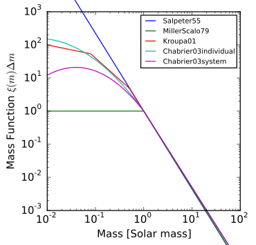
The image above shows a number of popular initial mass functions. The BPASS initial mass functions most closely resemble Kroupa01, in that we have three linear functions that are defined over different mass ranges and stitched together at the boundaries of each interval. We believe this to be a practical choice of IMF, and it is simple to integrate later on in the code to determine $f_{MBBH}$.
Note: The BPASS models that we use contain a single simple stellar population (delta-function burst in star formation at time zero). We predict that this will limit the degree to which the models match the observed data, and we believe incorporating models with continuous star formation (which are available from BPASS) represents an area of further study.
Due to the nature of the data (there are many BPASS data files placed in a set of seven folders), we perform this process externally and pickle the resulting DataFrame. For the interested members of the audience, the data files may be found under “BROAD-BAND COLOURS - UBVRIJHKugriz” at http://bpass.auckland.ac.nz/2.html. Locally, we have stored these files in our DataRepo folder.
# ind: number of IMF slope combinations (number of blue links on BPASS website)
for i in range(len(ind)):

    os.chdir('/afs/cas.unc.edu/classes/fall2016/astr_703_001/bonfield/group_project/
              BPASS_mags/BPASSv2_'+ind[i]+'/OUTPUT_POP/'+key+'/')
    # print os.getcwd()     # check that we are moving through directories

    dat_files = glob.glob('*.dat')
    mod1,mod2,mod3,mod4,mod5,mod6,mod7 = [],[],[],[],[],[],[]
    df_sub = [mod1, mod2, mod3, mod4, mod5, mod6, mod7]
    df1,df2,df3,df4,df5,df6,df7,df8,df9,df10,df11 = [],[],[],[],[],[],[],[],[],[],[]
    df_arr = [df1, df2, df3, df4, df5, df6, df7, df8, df9, df10, df11]

    df_sub[i] = pd.DataFrame()

    for j in range(len(dat_files)):

        bpass = np.genfromtxt(dat_files[j],delimiter='',dtype=float)
        # pull out metallicity from data file name (start/stop are index positions)
        if key == 'binary':
            start = 13
            stop = 16
        elif key == 'single':
            start = 9
            stop = 12
        metallicity = float(dat_files[j][start:stop])/1000.

        age = bpass[:,0]
        metallicity = metallicity*np.ones(len(age))
        imf_1 = imf1[i]*np.ones(len(age))
        imf_2 = imf2[i]*np.ones(len(age))
        imf_3 = imf3[i]*np.ones(len(age))

        df_arr[j] = pd.DataFrame()

        df_arr[j]['IMF (0.1-0.5)'] = pd.Series(imf_1)
        df_arr[j]['IMF (0.5-100)'] = pd.Series(imf_2)
        df_arr[j]['IMF (100-300)'] = pd.Series(imf_3)
        df_arr[j]['Metallicity'] = pd.Series(metallicity)
        df_arr[j]['log(Age)'] = pd.Series(age)
        df_arr[j]['u'] = pd.Series(bpass[:,10])
        df_arr[j]['g'] = pd.Series(bpass[:,11])
        df_arr[j]['r'] = pd.Series(bpass[:,12])
        df_arr[j]['i'] = pd.Series(bpass[:,13])
        df_arr[j]['z'] = pd.Series(bpass[:,14])
        df_arr[j]['J'] = pd.Series(bpass[:,7])
        df_arr[j]['H'] = pd.Series(bpass[:,8])
        df_arr[j]['K'] = pd.Series(bpass[:,9])
# Read in the BPASS model data
bpass_single = pd.read_pickle('bpass_sin_mags.pkl')
bpass_binary = pd.read_pickle('bpass_bin_mags.pkl')

# Display data frame for binary models as example
bpass_binary.head()
| IMF (0.1-0.5) | IMF (0.5-100) | IMF (100-300) | Metallicity | log(Age) | u | g | r | i | z | J | H | K | |
|---|---|---|---|---|---|---|---|---|---|---|---|---|---|
| 0 | -1.3 | -2.0 | -2.0 | 0.001 | 6.0 | -16.72410 | -15.25659 | -14.97677 | -14.81755 | -14.64745 | -14.35990 | -14.23688 | -14.12323 |
| 1 | -1.3 | -2.0 | -2.0 | 0.001 | 6.1 | -16.89995 | -15.43458 | -15.15283 | -14.99264 | -14.82397 | -14.54499 | -14.42667 | -14.31568 |
| 2 | -1.3 | -2.0 | -2.0 | 0.001 | 6.2 | -17.12357 | -15.66747 | -15.39094 | -15.23271 | -15.06762 | -14.79439 | -14.68084 | -14.57534 |
| 3 | -1.3 | -2.0 | -2.0 | 0.001 | 6.3 | -17.60489 | -16.40239 | -16.45614 | -16.59758 | -16.69958 | -16.89289 | -17.24655 | -17.36608 |
| 4 | -1.3 | -2.0 | -2.0 | 0.001 | 6.4 | -17.63741 | -16.54304 | -16.77804 | -17.05414 | -17.24676 | -17.56112 | -18.00511 | -18.15740 |
2. Model Calculations
For each model under consideration, we have four parameters that provide us with our model grid for BPASS:
- Age
- Metallicity
- IMF Slopes (proxy for \(f_{MBBH}\))
- \(\alpha\) (binary fraction) : 0.0, 0.1, 0.2, 0.3, 0.4, 0.5, 0.6, 0.7, 0.8, 0.9, 1.0
- We mix the BPASS models in a manner such that \(\alpha\) of our population is binary stars, while \((1-\alpha)\) is single stars.
# combine magnitudes based on alpha (binary fraction)
def combine_mags(single,binary,alpha):

    single = np.array(single)
    binary = np.array(binary)
    return -2.5 * np.log10((alpha * 10**(-0.4*binary))+(1. - alpha) * (10**(-0.4*single)))
Each combination of these parameters defines a unique model with a set of model magnitudes. We must first scale these values to put ourselves on the same footing as our RESOLVE galaxies, with the normalization providing an estimate of the galaxy mass. Before we do, however, we will discuss how we compute \(f_{MMBH}\).
(2.1) Fraction of Massive Binary Black Holes
The fundamental science question that we address in this project pertains to the fraction of massive binary black holes in dwarf galaxies (\(f_{MBBH}\)) that would be massive enough to emit gravitational waves that could be detected by Earth-based gravitational wave detectors. For each model, we can calculate this parameter using the BPASS initial mass functions and alpha parameter.
We define the following piecewise function for the initial mass functions from BPASS:
where \((a,b,c)\) are the IMF slopes in the corresponding intervals (provided by BPASS) and \((C_1,C_2,C_3)\) are unknown constants.
Making use of the mass normalization condition (all IMFs are normalized to \(10^6 M_{\odot}\)) and boundary conditions, we are able to solve for the unknown constants. Once the system is solved, we can integrate the first moment of the IMF from \(90M_{\odot}\) (progenitor cutoff is from Belczynski et al.) to \(300M_{\odot}\) in order to find the fraction of (potential) massive binary black holes in our binary star population. To find \(f_{MBBH}\) (which is the fraction of massive binary black holes in the total population), we merely multiply the result from evaluating the integral under the curve by the binary fraction, \(\alpha\).
In summary, we walk away with \(f_{MBBH}\) for each unique combination of IMF slopes and alpha (70).
"""
Function to calculate fraction of massive progenitors in binaries.
Uses IMF slopes and alpha (binary fraction). The numerator is the integral
of the binary IMF integrated from 90 M_sun (massive progenitor cutoff from
Belczynski et. al. 2016) through 300 M_sun. The denominator is the
normalized mass of the model (10^6 M_sun).
"""
def fbin_calc(alpha, a, b, c):
    import scipy

    def intercept2(a, b, c):
        return ((1./(0.5*(300.**2-0.1**2)))*(10**6 - (1./3.)*a*(0.5**3 - 0.1**3) - (1./3.)*b*(100**3 - 0.5**3)
               - (1./3.)*c*(300**3 - 100**3) - (b-a)*0.5*(0.5*(0.5**2-0.1**2)) - (b-c)*(100.0)*(0.5*(300**2-100**2))))

    def imf2(x):
        return (b*x + yint2)*alpha

    def imf3(x):
        return (c*x + yint3)*alpha

    yint2 = intercept2(a, b, c)
    yint1 = (b-a)*(0.5) + yint2
    yint3 = (b-c)*(100.) + yint2

    a1 = float(scipy.integrate.quad(imf2, 90, 100)[0])
    a2 = float(scipy.integrate.quad(imf3, 100, 300)[0])

    f_bin = (a1+a2)/(10.**6)

    return f_bin
(2.2) Normalization and Chi-Squared
- BPASS models are based on instantaneous formation of stars with a total mass of \(10^6 M_{\odot}\).
- Since galaxies in RESOLVE contain far more mass than \(10^6 M_{\odot}\), we must normalize. To do so, we assume that the uncertainties on the model magnitudes are Poissonian when converted to fluxes, then perform the normalization in flux units (this is the natural linear scale for light output).
# convert RESOLVE absolute mags to fluxes
gfluxs = 10**(-0.4*gmags)

# upper - lower bound on flux error
hfluxs = 10**(-0.4*(gmags+errs))
lfluxs = 10**(-0.4*(gmags-errs))
errs = 0.5*(hfluxs - lfluxs)
We define the normalization to be the scale factor that minimizes \({\chi}^2\), where \({x_i}\) are the model fluxes, \({d_i}\) are the observed (RESOLVE) fluxes, \({\epsilon_i}\) are the observed (RESOLVE) uncertainties, and \(i\) is the band index. We display the result below:
- After normalizing the model fluxes with this factor, we compute \({\chi}^2\) using normalized model magnitudes and observed magnitudes (with uncertainties) for each model.
- We later use \({\chi}^2\) to determine the posterior probability of each model for a given galaxy.
The code for carrying out this process takes a bit of a long time to run, so we have extracted another block of code from our pipeline to demonstrate how we compute normalizations and \({\chi}^2\) values.
# store useful strings in arrays for later
rmag_list = ['umag','gmag','rmag','imag','zmag','2jmag','2hmag','2kmag']
emag_list = ['e_umag','e_gmag','e_rmag','e_imag','e_zmag','e_2jmag','e_2hmag','e_2kmag']
bmag_list = ['u','g','r','i','z','J','H','K']

# compute interesting values for one galaxy
# parallelize at the individual galaxy level
numProcs = multiprocessing.cpu_count()

def out_calc(gal):
    # determine all the galaxy level variables
    # a few galaxies throw errors due to missing data
    # skip those with try - except statement
    try:
        # set scope of output_arr
        output_arr = []
        # extract error values from RESOLVE
        errs =[]
        for eband in emag_list:
            # only add good values to list
            if (gal[eband] != -99.0):
                errs.append(gal[eband])
        num_good_values = len(errs)

        # add 0.1 mag to all errors Kannappan (2007)
        errs = np.array(np.sqrt(np.array(errs)**2 + 0.1**2))

        # extract apparent RESOLVE magnitudes
        gmags = []
        for gband in rmag_list:
            # only add good values to list
            if (gal[gband] != -99.0):
                gmags.append(gal[gband])
        gmags = np.array(gmags)

        # distance to galaxy (grcz over cz due to additional corrections)
        distance = gal['grpcz'] / (70. / 10**6)

        # convert RESOLVE apparent magnitudes to absolute magnitudes
        gal_abs_mags = gmags - 5.0*np.log10(distance/10.0)
        gmags = gal_abs_mags

        # convert RESOLVE absolute mags to fluxes
        gfluxs = 10**(-0.4*gmags)

        # upper - lower bound on flux error
        hfluxs = 10**(-0.4*(gmags+errs))
        lfluxs = 10**(-0.4*(gmags-errs))
        errs = 0.5*(hfluxs - lfluxs)

        # loop over binary fraction
        for alpha in np.arange(0.0, 1.1, .1):
            # list of absolute magnitude vectors
            mags = combine_mags(bpass_single[bmag_list[:num_good_values]], bpass_binary[bmag_list
                               [:num_good_values]],alpha)
            # set arrays for normilaztion and chi-square
            norms = np.zeros(len(mags))
            chi2 = np.zeros(len(mags))
            for k, mmags in enumerate(mags):
                # select mag vector for model and convert model mags to fluxes
                mfluxes = 10**(-0.4*mmags)
                # compute norm and chi-square
                norms[k] = np.sum((gfluxs*mfluxes)/errs**2)/np.sum((mfluxes/errs)**2)
                chi2[k] = np.sum((gfluxs-norms[k]*mfluxes)**2/errs**2)/num_good_values

                # extract model information (to be used later)
                imf1 = bpass_single.iloc[k]['IMF (0.1-0.5)']
                imf2 = bpass_single.iloc[k]['IMF (0.5-100)']
                imf3 = bpass_single.iloc[k]['IMF (100-300)']
                age = bpass_single.iloc[k]['log(Age)']
                metallicity = bpass_single.iloc[k]['Metallicity']
                output_list = [gal['name'], imf1, imf2, imf3, age, metallicity, alpha, norms[k],
                               chi2[k],num_good_values]
                output_arr.append(output_list)
        print(output_list)
    except:
        print('A problem occured for %s' %gal['name'])

    return output_arr

pool = multiprocessing.Pool(numProcs-1)
# generate list of all dwarfs in RESOLVE for calculation
gal_list = [gal for index, gal in resolve.iterrows()]
output = pool.map(out_calc, gal_list)
# the output will be a list of lists of lists ordered by galaxy. Flatten to one giant list of lists
# each list is a model
merged = list(itertools.chain.from_iterable(output))
# convert to a dataframe for saving
df = pd.DataFrame(merged, columns = output_columns)
df.to_csv('all_output.csv', index=False)
# Load in data for a couple of galaxies of choice.
bpass = pd.read_csv('output_three.csv')
#
'''
# UNCOMMENT IF YOU WISH TO CALCULATE F_MBBH MANUALLY.

# Initialize array to store f_{MBBH} for each model.
fmbbh = np.zeros(len(bpass.index))

# Add a column to the data frame for f_{MBBH}.
for index, row in bpass.iterrows():
    imf1 = row['IMF (0.1-0.5)']
    imf2 = row['IMF (0.5-100)']
    imf3 = row['IMF (100-300)']
    alpha_gal = row['Alpha']
    fmbbh[index] = fbin_calc(alpha_gal, imf1, imf2, imf3)

bpass['f_{MBBH}'] = fmbbh
'''

bpass.head()
| Name | IMF (0.1-0.5) | IMF (0.5-100) | IMF (100-300) | log(Age) | Metallicity | Alpha | Normalization | Chi^2 | Good Bands | |
|---|---|---|---|---|---|---|---|---|---|---|
| 0 | rf0044 | -1.3 | -2.0 | -2.0 | 6.0 | 0.001 | 0.0 | 2.076575 | 57.360405 | 8 |
| 1 | rf0044 | -1.3 | -2.0 | -2.0 | 6.1 | 0.001 | 0.0 | 1.790453 | 57.377654 | 8 |
| 2 | rf0044 | -1.3 | -2.0 | -2.0 | 6.2 | 0.001 | 0.0 | 1.536136 | 57.342386 | 8 |
| 3 | rf0044 | -1.3 | -2.0 | -2.0 | 6.3 | 0.001 | 0.0 | 1.068513 | 52.654002 | 8 |
| 4 | rf0044 | -1.3 | -2.0 | -2.0 | 6.4 | 0.001 | 0.0 | 1.287277 | 28.877582 | 8 |
(2.3) Galaxy-Specific Calculations
With the models defined, we can compute from the normalizations an estimate for \(M_*, \alpha \), metallicity, and age for each galaxy. In order to compare to the RESOLVE mass for each galaxy, we compute the median (as done by previous works, Kannappan and Gawiser 2007) and the median weighted by the likelihood of each model (new approach?).
(2.3a) Computing the Model-Weighted Parameters for Each Galaxy
input_df = pd.read_csv('output_three.csv')
galaxy_names = np.unique(input_df['Name'])
# Define the weighted mean function.
def weighted_median(values, weights):
'''
Compute the weighted median of values list.
The weighted median is computed as follows:
1- sort both lists (values and weights) based on values, then
2- select the 0.5 point from the weights and return the
corresponding values as results.
e.g. values = [1, 3, 0] and weights=[0.1, 0.3, 0.6], assuming
weights are probabilities.
sorted values = [0, 1, 3] and corresponding sorted
weights = [0.6, 0.1, 0.3]. The 0.5 point on weight corresponds
to the first item which is 0., so the weighted median is 0.
'''
# convert the weights into probabilities
sum_weights = sum(weights)
weights = np.array([(w*1.0)/sum_weights for w in weights])
# sort values and weights based on values
values = np.array(values)
sorted_indices = np.argsort(values)
values_sorted = values[sorted_indices]
weights_sorted = weights[sorted_indices]
# select the median point
it = np.nditer(weights_sorted, flags=['f_index'])
accumulative_probability = 0
median_index = -1
while not it.finished:
accumulative_probability += it[0]
if accumulative_probability > 0.5:
median_index = it.index
return values_sorted[median_index]
elif accumulative_probability == 0.5:
median_index = it.index
it.iternext()
next_median_index = it.index
return np.mean(values_sorted[[median_index, next_median_index]])
it.iternext()
return values_sorted[median_index]
# define galaxy independent variables
range_z = 0.04-0.001
range_logA = 10.0-6.0
priors = range_z**-1*range_logA**-1
dpz = range_z/11.0
dplA = range_logA/41.0
ages = np.array(input_df[ (input_df['Name'] == galaxy_names[0]) ]['log(Age)'])
Zs = np.array(input_df[ (input_df['Name'] == galaxy_names[0]) ]['Metallicity'])
alphas = np.array(input_df[ (input_df['Name'] == galaxy_names[0]) ]['Alpha'])
output_columns = ['Name', 'walpha', 'wage', 'wZ','median', 'wmean', 'wmedian','logmstar',
'diff', '%diff']
def analyze_mass(galaxy):
"""
:param galaxy: name of galaxy from input_df
:return: output_list
"""
norms = np.array(input_df[ (input_df['Name'] == galaxy) ]['Normalization'])
chis = np.array(input_df[ (input_df['Name'] == galaxy) ]['Chi^2'])
# implement a scale factor for better numerical results. Same accros all galaxies
chis = chis/10.0
lnprobs = -0.5*chis + np.log(priors)
probs = np.exp(lnprobs)
logmstar = np.array(resolve[(resolve['name'] == galaxy)]['logmstar'])[0]
ratios = norms
logmass = np.log10(ratios*10**6)
# calculate weighted values
wmean = np.sum(np.exp(-chis*0.5)*logmass)/np.sum(np.exp(-chis*0.5))
wmedian = weighted_median(logmass, probs/np.sum(probs))
walpha = np.sum(np.exp(-chis*0.5)*alphas)/np.sum(np.exp(-chis*0.5))
wage = np.sum(np.exp(-chis*0.5)*ages)/np.sum(np.exp(-chis*0.5))
wZ = np.sum(np.exp(-chis*0.5)*Zs)/np.sum(np.exp(-chis*0.5))
# generate output line
output_list = [galaxy,walpha,wage,wZ,np.median(logmass),wmean,wmedian,
logmstar,logmstar-wmedian,((logmstar-wmedian)/logmstar)*100.0]
print(output_columns)
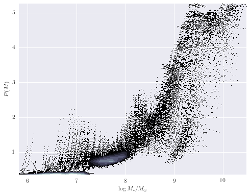
# output mass - probability plot
fig, ax = plt.subplots(figsize=(8, 6))
scatter_contour(logmass, probs, threshold=200, log_counts=True, ax=ax,
histogram2d_args=dict(bins=40),
plot_args=dict(marker=',', linestyle='none', color='black'),
contour_args=dict(cmap=plt.cm.bone))
ax.set_xlabel(r'${\log M_*/M_{\odot}}$')
ax.set_ylabel(r'${P(M)}$')
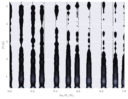
# output alpha - probability plot
fig, ax = plt.subplots(figsize=(8, 6))
scatter_contour(alphas, probs, threshold=20, log_counts=False, ax=ax,
histogram2d_args=dict(bins=40),
plot_args=dict(marker=',', linestyle='none', color='black'),
contour_args=dict(cmap=plt.cm.bone))
ax.set_xlabel(r'${\alpha}$')
ax.set_ylabel(r'${P(M)}$')
return output_list
analyze_mass(galaxy_names[0])
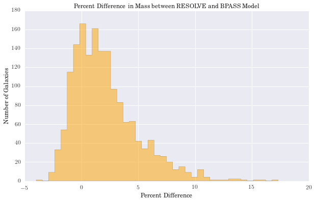
(2.3b) Mass Comparison with RESOLVE
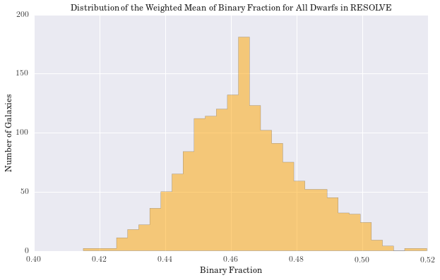
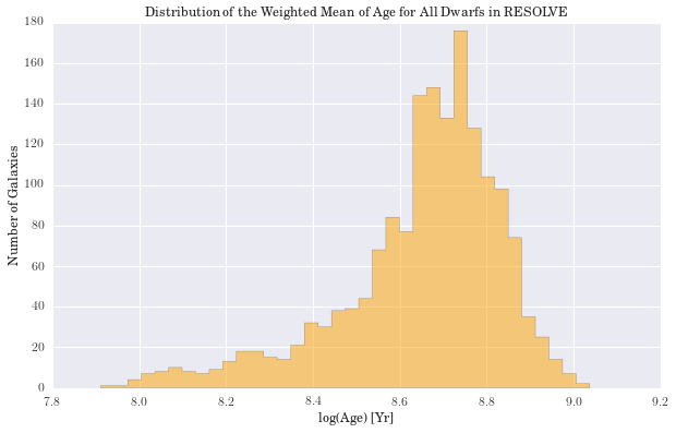
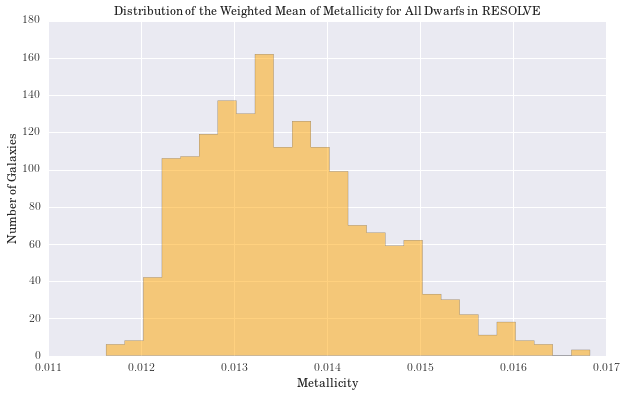
We have computed the percent difference between logmstar in RESOLVE and our weighted median calculation for all galaxies. We see the largest difference is 17%, but this is in a small tail of the distribution (if centered on zero), suggesting good agreement with RESOLVE. Results for age and metallicity are also as expected. For the fraction of binaries, \(\alpha\), we see a narrow band centered around 40%. This is an encouraging result, as it has been estimated that up to 70% of stars may be participating in binary interactions. Therefore, these models suggest SPS models would better fit galaxy spectra with a significant fraction of binary stars.
In exploring our data, we noticed that as the fraction of binary stars was increased, estimates for galaxy mass tended to increase as well. Eldridge and Stanway (2016) suggest supermassive binary black holes will only develop in very low metallicity environments. While the weighted metallicity results are low in the range of these models, they are still too high to be strong candidates for these types of objects.
# load input data frame for each galaxy
massframe = pd.read_csv('galaxy_analysis.csv')

# extract interesting values to numpy arrays for graphing
masses = np.array(massframe['wmedian'])[:, np.newaxis]
resolve_masses = np.array(massframe['logmstar'])
diffs = np.array(massframe['%diff'])
walphas = np.array(massframe['walpha'])
wages = np.array(massframe['wage'])
wZs = np.array(massframe['wZ'])

# worst prediction
print('Largest percent difference in mass: %2.2f' %np.max(massframe['%diff']))

# distribution of differences with RESOLVE
plt.figure(figsize=(10, 6))
counts, bins, patches = hist(diffs, bins='knuth', color='orange', histtype='stepfilled', normed=False, alpha=0.5)
plt.xlabel("Percent Difference")
plt.ylabel("Number of Galaxies")
plt.title('Percent Difference in Mass between RESOLVE and BPASS Model')
#plt.show()

# distribution of weighted alphas
plt.figure(figsize=(10, 6))
counts, bins, patches = hist(walphas, bins='knuth', color='orange', histtype='stepfilled', normed=False, alpha=0.5)
plt.xlabel("Binary Fraction")
plt.ylabel("Number of Galaxies")
plt.title('Distribution of the Weighted Mean of Binary Fraction for All Dwarfs in RESOLVE')
#plt.show()

# distribution of weighted ages
plt.figure(figsize=(10, 6))
counts, bins, patches = hist(wages, bins='knuth', color='orange', histtype='stepfilled', normed=False, alpha=0.5)
plt.xlabel("log(Age) [Yr]")
plt.ylabel("Number of Galaxies")
plt.title('Distribution of the Weighted Mean of Age for All Dwarfs in RESOLVE')
#plt.show()

# distribution of weighted metallicities
plt.figure(figsize=(10, 6))
counts, bins, patches = hist(wZs, bins='knuth', color='orange', histtype='stepfilled', normed=False, alpha=0.5)
plt.xlabel("Metallicity")
plt.ylabel("Number of Galaxies")
plt.title('Distribution of the Weighted Mean of Metallicity for All Dwarfs in RESOLVE')
#plt.show()
Largest percent difference in mass: 17.30
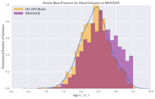
(2.3c) Cross-Validation and the Stellar Mass Function
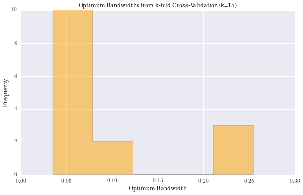
We have computed the stellar mass function of the dwarf galaxies in RESOLVE using Kernel Density Estimation. The bandwidth of the kernel was determined using k-fold cross-validation with k=15.
# Perform k-fold cross-validation
mass_arr = masses[:,0]
np.random.shuffle(mass_arr)
mass_arr = mass_arr[:1650]

# determine Knuth's optimal bin size for the entire data set
knuthBinWidth = astropy.stats.knuth_bin_width(mass_arr)
print('The Knuth optimal bin width is: %f' % knuthBinWidth)
bandwidths = np.arange(0.4 * knuthBinWidth, 3.0 * knuthBinWidth, 0.01)

# split the data into 15 subsets
num_splits = 15
optimum_widths = np.zeros(num_splits)
kfold_arr = np.split(mass_arr, num_splits)

for run in range(num_splits):
    mask = np.ones(num_splits, dtype=bool)
    mask[run] = False
    test_data = kfold_arr[run]
    train_data = np.delete(kfold_arr, run, axis=0).flatten()

    logLs = np.zeros(bandwidths.size)
    for j, bandwidth in enumerate(bandwidths):
        # KDE
        kde = KernelDensity(kernel='gaussian', bandwidth=bandwidth).fit(train_data[:, np.newaxis])
        logLs[j] = kde.score(test_data[:, np.newaxis])
        optimum_widths[run] = bandwidths[np.argmax(logLs)]

widths = np.unique(optimum_widths)

print('------------RESULTS----------------------')
print('The median value of bandwidths is: %f' % np.median(optimum_widths))
print('The mean value of bandwidths is: %f' % np.mean(optimum_widths))
print('The std dev of bandwidths is: %f' % np.std(optimum_widths, ddof=1))
plt.figure(figsize=(10, 6))
counts, bins, patches = hist(optimum_widths, bins='knuth', color='orange',
                             histtype='stepfilled', normed=False, alpha=0.5)
plt.xlabel("Optimum Bandwidth")
plt.ylabel("Frequency")
plt.title('Optimum Bandwidths from k-fold Cross-Validation (k=15)')
#plt.show()

# choose KDE bandwidth with k-fold median
kde = KernelDensity(kernel='gaussian', bandwidth=np.mean(widths)).fit(masses)
mass_plot = np.linspace(7.0,10,len(masses))[:, np.newaxis]
log_dens = kde.score_samples(mass_plot)
f = np.exp(log_dens)

plt.figure(figsize=(10, 6))
counts, bins, patches = hist(masses[:,0], bins='knuth', color='orange', histtype='stepfilled',
                             label='DG SPS Model',normed=True, alpha=0.5)
counts, bins, patches = hist(resolve_masses, bins='knuth', color='purple', histtype='stepfilled',
                             label='RESOLVE',normed=True, alpha=0.5)
plt.xlabel("log($M_{*}/M_{\odot}$)")
plt.ylabel("Normalized Number of Galaxies")
plt.legend(loc=2)
plt.title('Stellar Mass Function for Dwarf Galaxies in RESOLVE')
plt.plot(mass_plot[:,0], f, '-')
#plt.show()
The Knuth optimal bin width is: 0.087364
------------RESULTS----------------------
The median value of bandwidths is: 0.074946
The mean value of bandwidths is: 0.099612
The std dev of bandwidths is: 0.079988
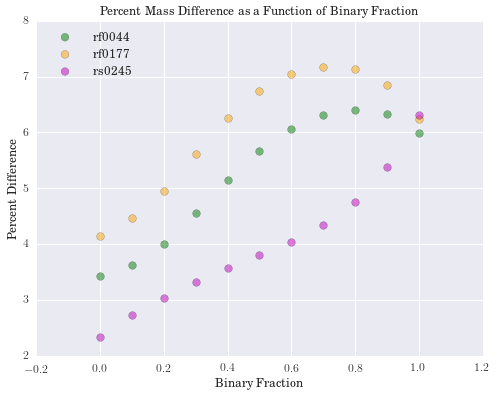
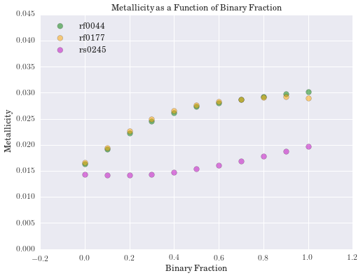
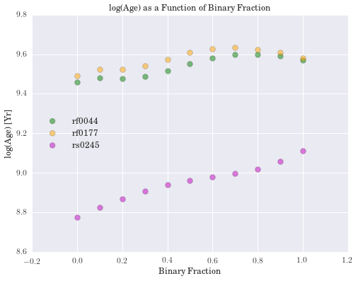
(2.3d) Galaxy Parameters as a Function of Binary Fraction
To further investigate our fundamental question, we explored how our galaxy parameters behave as a function of the binary fraction (as opposed to \(f_{MBBH}\)). To do so, we chose three dwarf galaxies with different mass estimates from RESOLVE to capture what we felt was a representative (albeit small) picture of how our code runs for the entire sample.
# Load data for three galaxies.
df = pd.read_csv('output_three.csv')

# Select the galaxy names to loop over.
galaxy_names = np.unique(df['Name'])

# Do calculations for the first galaxy.
norms = df[ (df['Name'] == galaxy_names[0]) ]['Normalization']
chis = df[ (df['Name'] == galaxy_names[0]) ]['Chi^2']
range_z = 0.04-0.001
range_logA = 10.0-6.0
priors = range_z**-1*range_logA**-1
dpz = range_z/11.0
dplA = range_logA/41.0
lnprobs = -0.5*chis + np.log(priors)
probs = np.exp(lnprobs)
ages = df[ (df['Name'] == galaxy_names[0]) ]['log(Age)']
Zs = df[ (df['Name'] == galaxy_names[0]) ]['Metallicity']
alphas = df[ (df['Name'] == galaxy_names[0]) ]['Alpha']
cz = resolve[(resolve['name'] == galaxy_names[0])]['cz']
logmstar = resolve[(resolve['name'] == galaxy_names[0])]['logmstar']
ratios = norms
logmass = np.log10(ratios*10**6)

# Calculate mass difference as a function of alpha.
def diff_alpha(gal_name, alphas=alphas):
    alphas = np.unique(alphas)
    wmalpha = np.zeros(len(alphas))
    diffs = np.zeros(len(alphas))
    metal = np.zeros(len(alphas))
    age = np.zeros(len(alphas))
    for k, alpha in enumerate(alphas):
        # dataframe centric structure
        temp = df[ (df['Name'] == gal_name) & (df['Alpha'] == alpha)]
        ntemp = len(temp)
        ptemp = np.zeros(ntemp)
        mtemp = np.zeros(ntemp)
        j = 0
        for index, row in temp.iterrows():
            mass = np.log10(row['Normalization']*10**6)
            lnprob = -0.5*row['Chi^2'] + np.log(priors)
            prob = np.exp(lnprob)
            ptemp[j] = prob
            mtemp[j] = mass
            j += 1

        mtemp = pd.Series(mtemp)
        ptemp = pd.Series(ptemp)

        temp = temp.assign(mass = mtemp.values)
        temp = temp.assign(prob = ptemp.values)
        logmstar = resolve[(resolve['name'] == gal_name)]['logmstar']

        wmalpha[k] = np.sum(temp['prob']*temp['mass'])/np.sum(temp['prob'])
        diffs[k] = (wmalpha[k] - logmstar)/logmstar*100.0
        metal[k] = np.sum(temp['prob']*temp['Metallicity'])/np.sum(temp['prob'])
        age[k] = np.sum(temp['prob']*temp['log(Age)'])/np.sum(temp['prob'])
    return diffs,metal,age

run1 = diff_alpha(galaxy_names[0])
run2 = diff_alpha(galaxy_names[1])
run3 = diff_alpha(galaxy_names[2])

plt.figure(figsize=(8,6))
plt.scatter(np.unique(alphas), run1[0], s=60, c='g', alpha=0.5)
plt.scatter(np.unique(alphas), run2[0], s=60, c='orange', alpha=0.5)
plt.scatter(np.unique(alphas), run3[0], s=60, c='m', alpha=0.5)
plt.legend(galaxy_names, loc=2)
plt.xlabel("Binary Fraction")
plt.ylabel("Percent Difference")
plt.title('Percent Mass Difference as a Function of Binary Fraction')

plt.figure(figsize=(8,6))
plt.scatter(np.unique(alphas), run1[1], s=60, c='g', alpha=0.5)
plt.scatter(np.unique(alphas), run2[1], s=60, c='orange', alpha=0.5)
plt.scatter(np.unique(alphas), run3[1], s=60, c='m', alpha=0.5)
plt.legend(galaxy_names, loc=2)
plt.xlabel("Binary Fraction")
plt.ylabel("Metallicity")
plt.title('Metallicity as a Function of Binary Fraction')
plt.show()

plt.figure(figsize=(8,6))
plt.scatter(np.unique(alphas), run1[2], s=60, c='g', alpha=0.5)
plt.scatter(np.unique(alphas), run2[2], s=60, c='orange', alpha=0.5)
plt.scatter(np.unique(alphas), run3[2], s=60, c='m', alpha=0.5)
plt.legend(galaxy_names, loc=6)
plt.xlabel("Binary Fraction")
plt.ylabel("log(Age) [Yr]")
plt.title('log(Age) as a Function of Binary Fraction')
plt.show()
(2.4) Bayesian Analysis
Up until this point, we have not performed any calculations that require any sort of formal Bayesian analysis. That is, we have not imposed priors on the model parameters with the hope of getting an idea of which ones are best for a given galaxy (nor have we discussed an appropriate likelihood function or performed any sort of marginalization). We include a brief discussion of each below, followed by code to demonstrate how this works for our sample galaxy.
(2.4a) Priors
- IMF slopes: We do not claim to know anything about these parameters a priori, so we do not incorporate anything into our prior that pertains to IMF slopes.
- We will also not marginalize to capture the posterior distribution for these parameters.
- Age: We impose a uniform prior on
log(Age), spanning the range of ages provided by BPASS.- Although we could probably define a better prior here, we did not want to chop off any viable ages on accident.
- Metallicity: We impose a uniform prior on
Metallicity, spanning the range of metallicities provided by BPASS. - Alpha: We impose a uniform prior on
alpha, spanning the range of binary fractions that we test.- Note: Since this is just one, we do not include it explicitly below.
Our prior distribution is given below, where \({\theta}_i\) represents our set of model parameters.
(2.4b) Likelihood Function
We believe our problem motivates the use of a likelihood function that depends on the chi-squared distribution, as discussed previously. Therefore, our likelihood function is of the form:
where \(f_{B,i}\) are the normalized BPASS fluxes, \(f_{R,i}\) are the RESOLVE fluxes, and \(\sigma_{R,i}\) are the RESOLVE flux uncertainties.
(2.4c) Marginalization
To examine the parameters of interest (age, metallicity, alpha), we must marginalize over the nuisance parameters (i.e., the ones that are not of interest to us). We perform this in the usual manner (summing over particular axis/axes in our DataFrame, then normalizing). We do this for a single galaxy, but this code can be extended to the entire sample.
# Load in data for a couple of galaxies of choice.
bpass = pd.read_pickle('output_two.pkl')
# Define useful set of arrays for later.
log_ages = np.arange(6.0,10.1,0.1)
metallicities = np.array([0.001, 0.002, 0.003, 0.004, 0.006, 0.008, 0.010,
0.014, 0.020, 0.030,0.040])
alphas = np.arange(0.0,1.1,0.1)
target_list = ['rf0001 '] # Note: To be specified by user.
# Future note: Could define functions below as a single function with option index.
'''
Marginalize over metallicities to get posterior distribution for age.
'''
def marginalize_age(df,targets,ages,metallicities,alphas):
marg_ages = np.zeros((int(len(targets)),np.size(ages),2))
range_z = np.max(metallicities) - np.min(metallicities)
range_logA = np.max(ages) - np.min(ages)
priors = range_z**-1*range_logA**-1
#dpz = range_z/np.size(metallicities)
dplA = range_logA/np.size(ages)
chis = df['Chi^2']
prob = np.sum(np.exp(-0.5*chis) + np.log(priors))
den = prob * dplA
for i, galaxy in enumerate(targets):
gal_df = df.loc[df['Name'] == galaxy]
for j, age in enumerate(ages):
ages_bool = np.isclose(gal_df['log(Age)'],age,1e-4)
ages_df = gal_df.loc[ages_bool]
gal_chis = ages_df['Chi^2']
gal_prob = np.sum(np.exp(-0.5*gal_chis) + np.log(priors))
marg_ages[i,j,0] = age
marg_ages[i,j,1] = gal_prob / den
return marg_ages
'''
Marginalize over ages to get posterior distribution for metallicity.
'''
def marginalize_metallicity(df,targets,ages,metallicities,alphas):
marg_metals = np.zeros((int(len(targets)),np.size(metallicities),2))
range_z = np.max(metallicities) - np.min(metallicities)
range_logA = np.max(ages) - np.min(ages)
priors = range_z**-1*range_logA**-1
dpz = range_z/np.size(metallicities)
#dplA = range_logA/np.size(ages)
chis = df['Chi^2']
prob = np.sum(np.exp(-0.5*chis) + np.log(priors))
den = prob * dpz
for i, galaxy in enumerate(targets):
gal_df = df.loc[df['Name'] == galaxy]
for j, metal in enumerate(metallicities):
metals_df = gal_df.loc[gal_df['Metallicity'] == metal]
gal_chis = metals_df['Chi^2']
gal_prob = np.sum(np.exp(-0.5*gal_chis) + np.log(priors))
marg_metals[i,j,0] = metal
marg_metals[i,j,1] = gal_prob / den
return marg_metals
'''
Marginalize over ages/metallicities to get posterior distribution for alpha.
'''
def marginalize_alpha(df,targets,ages,metallicities,alphas):
marg_alphas = np.zeros((int(len(targets)),np.size(alphas),2))
range_z = np.max(metallicities) - np.min(metallicities)
range_logA = np.max(ages) - np.min(ages)
priors = range_z**-1*range_logA**-1
#dpz = range_z/np.size(metallicities)
#dplA = range_logA/np.size(ages)
chis = df['Chi^2']
prob = np.sum(np.exp(-0.5*chis) + np.log(priors))
den = prob
for i, galaxy in enumerate(targets):
gal_df = df.loc[df['Name'] == galaxy]
for j, alpha in enumerate(alphas):
alphas_df = gal_df.loc[gal_df['Alpha'] == alpha]
gal_chis = alphas_df['Chi^2']
gal_prob = np.sum(np.exp(-0.5*gal_chis) + np.log(priors))
marg_alphas[i,j,0] = alpha
marg_alphas[i,j,1] = gal_prob / den
return marg_alphas
m_ages = marginalize_age(bpass,target_list,log_ages,metallicities,alphas)
m_mets = marginalize_metallicity(bpass,target_list,log_ages,metallicities,alphas)
m_alphs = marginalize_alpha(bpass,target_list,log_ages,metallicities,alphas)
plt.figure(4)
plt.clf()
plt.plot(m_ages[0,:,0],m_ages[0,:,1],'b.',markersize='10.')
plt.xlabel("log(Age) [Yr]")
plt.ylabel("Marginalized Posterior Distribution")
plt.figure(5)
plt.clf()
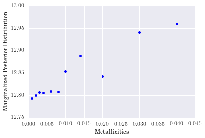
plt.plot(m_mets[0,:,0],m_mets[0,:,1],'b.',markersize='10.')
plt.xlabel("Metallicities")
plt.ylabel("Marginalized Posterior Distribution")
plt.figure(6)
plt.clf()
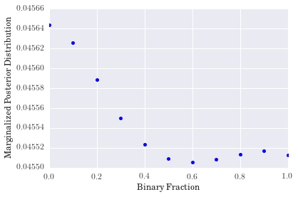
plt.plot(m_alphs[0,:,0],m_alphs[0,:,1],'b.',markersize='10.')
plt.xlabel("Binary Fraction")
plt.ylabel("Marginalized Posterior Distribution")
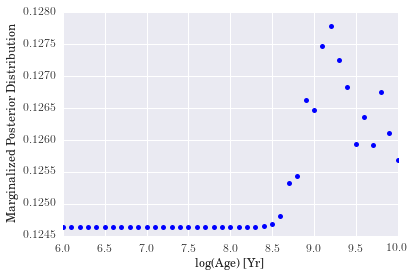
- We see that although the marginalized posterior distribution for age is peaked a little after 1 Gyr, there is some additional scatter near the edge of the distribution that would appear to indicate that we did not do an excellent job of capturing the age of the galaxy.
- For metallicity, our results indicate that a high-metallicity model is favored for
rf0001. Again, we see some non-monotonic behavior as metallicity increases, but we cannot conclude much because it looks as though a proper fit for the metallicity would fall beyond the extent of our model grid. - The distribution for binary fraction, however, appears to favor a low binary fraction for this particular galaxy. The degree to which it does so is somewhat surprising, but reasonable nonetheless.
3. Method Comparison
Initially, our group wished to use a variety of MCMC samplers in Python (emcee, PyStan) for our project, but we found the lack of an analytic model (that is, an analytic model that depends on all of our model parameters in a coherent fashion) made this task impossible. Instead, we decided to explore a number of different sampling algorithms for exploring our posterior distribution. We had moderate amounts of success with two of the methods, while the third/fourth ultimately did not work for our parameter space.
The motivation for sampling from this distribution is that our dataset could become computationally intensive if we were to add more complicated models, more galaxies, or just wanted to compute more quantities (i.e., it would not take much to blow up our parameter space). Without needing to perform calculations on the entire dataset, we explore three methods for sampling from our posterior. The goal of this sampling is to identify areas of interest in our parameter space and determine the expected distribution of the massive binary black hole fraction, $f_{MBBH}$, for individual galaxies.
Note: Due to the coarse nature of our model grid, our sampling algorithm had a relatively small parameter space to explore. Nevertheless, we hope to demonstrate the effictiveness of each.
(3.1) Simple Random Sampling
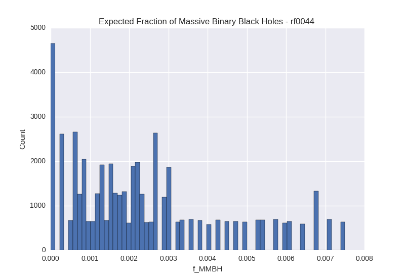
Since we have a rather complicated model space and little intuition as to where the “good” models will be, we first perform simple random sampling to sample from our posterior probability distribution. The advantage of this method is that each model has an equal probability of being selected and if performed multiple times, the samples are statistically independent. This method is additionally motivated by the fact that the marginalized posterior distributions are mostly featureless.
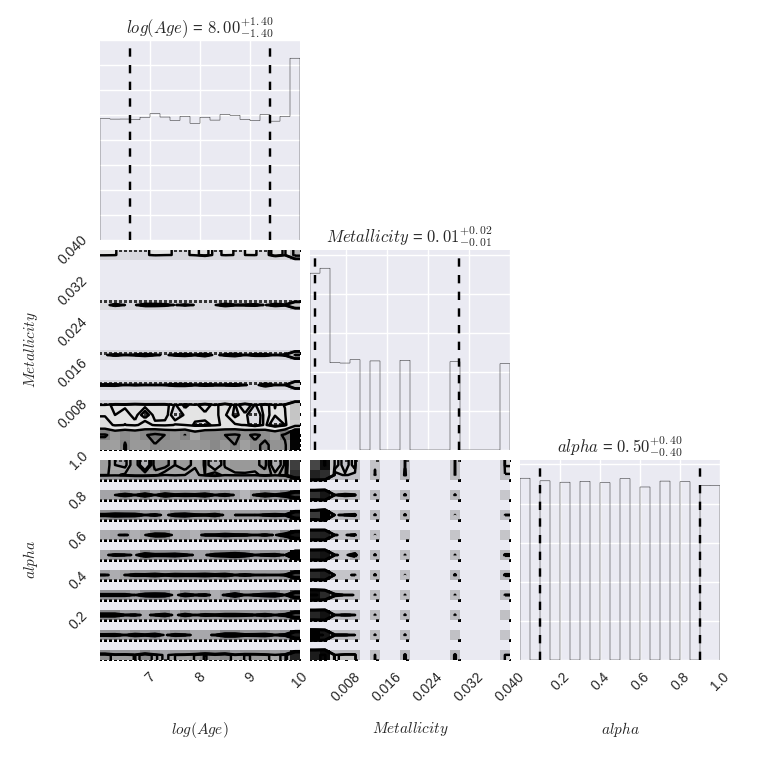
For each method, we generate a corner plot for the three parameters we are most interested in and display the median value and 16th/84th percentile values for each. We also plot a histogram of the calculated $f_{MBBH}$ values.
# Define values to randomly sample
all_names = ['rf0044 ', 'rf0177 ', 'rs0245 ']
all_age = np.arange(6.0,10.1,0.1)
all_z = np.array([0.001, 0.002, 0.003, 0.004, 0.006, 0.008, 0.010, 0.014, 0.020, 0.030, 0.040])
all_alpha = np.linspace(0.0,1.0,11)
all_imfs = np.array([ [-1.30, -2.0, -2.0], [-1.30, -2.0, 0.0], [-2.35, -2.35, 0.0],
                     [-1.30, -2.35, -2.35], [-1.30, -2.35, 0.0], [-1.30, -2.70, -2.70],
                     [-1.30, -2.70, 0.0] ])

# Function for computing posterior probability using previously stated prior.
def posterior_prob(p, chisq):
    range_z = 0.04-0.001
    range_logA = 10.0-6.0
    priors = range_z**-1*range_logA**-1
    lnprob = -0.5*chisq + np.log(priors)
    prob = np.exp(lnprob)
    return prob

# Reload RESOLVE data and model data.
resolve = pd.read_pickle('resolve.pkl')
resolve = resolve[(resolve['logmstar'] < 9.5)]
df = pd.read_csv('output_three.csv')

def sps_rand(gal):
    # Initially choose random point within the parameter space.
    imf_ind = np.random.randint(len(all_imfs))
    p_0 = [all_age[np.random.randint(len(all_age))],
           all_z[np.random.randint(len(all_z))],
           all_alpha[np.random.randint(len(all_alpha))],
           all_imfs[imf_ind][0],
           all_imfs[imf_ind][1],
           all_imfs[imf_ind][2]]

    # Steps in MCMC chain
    nsteps = 51000
    current_post_prob = 1e-15   # choose low initial values arbitrarily to get the chain moving
    current_fbin = 1e-10

    # Initialize arrays to store results from chain (originally set up to be used for multiple galaxies at once)
    gal_arr = resolve['name']
    age_arr = np.zeros((len(gal_arr), nsteps))
    z_arr = np.zeros((len(gal_arr), nsteps))
    alpha_arr = np.zeros((len(gal_arr), nsteps))
    imf1_arr = np.zeros((len(gal_arr), nsteps))
    imf2_arr = np.zeros((len(gal_arr), nsteps))
    imf3_arr = np.zeros((len(gal_arr), nsteps))
    prob_arr = np.zeros((len(gal_arr), nsteps))
    fbin_arr = np.zeros((len(gal_arr), nsteps))
for n in range(nsteps):
    print '------------------------------------------------------------------'
    print 'Galaxy: ', gal
    print 'Step number : ', n

    # Calculate new step, using normally distributed integers for each parameter
    imf_ind = np.random.randint(len(all_imfs))
    p_new = [all_age[np.random.randint(len(all_age))],
             all_z[np.random.randint(len(all_z))],
             all_alpha[np.random.randint(len(all_alpha))],
             all_imfs[imf_ind][0], all_imfs[imf_ind][1],
             all_imfs[imf_ind][2]]

    # Create boolean masks for each randomly selected parameter and "look up" the row that has those values
    name_bool = df['Name'] == gal
    age_bool = np.isclose(df['log(Age)'], p_new[0], 1e-4)
    z_bool = np.isclose(df['Metallicity'], p_new[1], 1e-4)
    alpha_bool = np.isclose(df['Alpha'], p_new[2], 1e-4)
    imf1_bool = np.isclose(df['IMF (0.1-0.5)'], p_new[3], 1e-4)
    imf2_bool = np.isclose(df['IMF (0.5-100)'], p_new[4], 1e-4)
    imf3_bool = np.isclose(df['IMF (100-300)'], p_new[5], 1e-4)

    current_row = df[name_bool & age_bool & z_bool & alpha_bool & imf1_bool & imf2_bool & imf3_bool]
    current_chisq = current_row['Chi^2']

    # Calculate posterior probability and m_bbh fraction at new point
    new_post_prob = posterior_prob([p_new[0], p_new[1]], current_chisq)
    parr = np.array(new_post_prob)
    new_post_prob = parr[0]

    new_fbin = fbin_calc(p_new[2], p_new[3], p_new[4], p_new[5])

    # If probability at new point is higher than old point, automatically accept
    # Add parameters and calculated values of new point
    gi=0
    age_arr[gi, n] = p_new[0]
    z_arr[gi, n] = p_new[1]
    alpha_arr[gi, n] = p_new[2]
    imf1_arr[gi, n] = p_new[3]
    imf2_arr[gi, n] = p_new[4]
    imf3_arr[gi, n] = p_new[5]
    prob_arr[gi, n] = new_post_prob
    fbin_arr[gi, n] = new_fbin

    current_post_prob = new_post_prob
    current_fbin = new_fbin
    p0 = p_new
    print p0
    print current_fbin

# Remove burn-in period (first 1000 steps)
zs = z_arr[0,1000:]
ages = age_arr[0,1000:]
alphas = alpha_arr[0,1000:]
fbins = fbin_arr[0,1000:]

# Corner plot of parameters from chain
plt.figure()
data = np.array([ages,zs,alphas]).T
corner.corner(data, labels=[r"$log(Age)$", r"$Metallicity$", r"$alpha$"], show_titles=True, quantiles=[0.16,0.84], plot_contours=True)
plt.savefig('corner_'+gal[0:-1]+'_random.png')
plt.clf()

# Histogram of f_mmbh calculated at each step in chain
plt.figure()
hist(fbins, bins='knuth')
plt.xlabel('f_MBBH')
plt.ylabel('Count')
plt.title('Expected Fraction of Massive Binary Black Holes - '+ gal)
plt.savefig('fbin_'+gal[0:-1]+'_random.png')
plt.clf()
# Simple Random Sampling - Corner Plot for Galaxy rf0044
Image("corner_rf0044_random.png")
# Simple Random Sampling - f_mmbh Histogram for Galaxy rf0044
Image("fbin_rf0044_random.png")
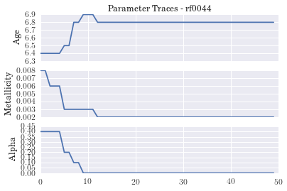
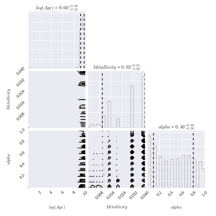
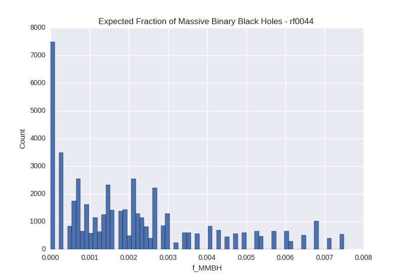
(3.2) Metropolis-Hastings Algorithm
Knowing we could do better than simple random sampling, we implemented a Metropolis-Hastings algorithm to generate a Markov Chain in our parameter space. This method takes advantage of most of the code used in the random sampler, with the addition of a conditional statement that calculates the posterior probability at each model point in the chain. We use the standard Metropolis-Hastings step criterion for determining whether or not to accept the next element in the chain. Additionally, we employ a Gaussian centered at the current point to select the following step candidate. Because our model grid is discrete and fairly coarse, this step calculation is not ideal. The results of this MCMC method would be improved if we were able to compute a function based on continuous parameters (and sample from a continuous parameter space). The computed values could also be more robust by using a bootstrapping method to calculate the mean and 1-sigma quantiles.
all_names = ['rf0044 ', 'rf0177 ', 'rs0245 ']
all_age = np.arange(6.0,10.1,0.1)
all_z = np.array([0.001, 0.002, 0.003, 0.004, 0.006, 0.008, 0.010, 0.014, 0.020, 0.030, 0.040])
all_alpha = np.linspace(0.0,1.0,11)
all_imfs = np.array([ [-1.30, -2.0, -2.0], [-1.30, -2.0, 0.0], [-2.35, -2.35, 0.0], [-1.30, -2.35, -2.35], [-1.30, -2.35, 0.0], [-1.30, -2.70, -2.70], [-1.30, -2.70, 0.0] ])

def posterior_prob(p, chisq):
    range_z = 0.04-0.001
    range_logA = 10.0-6.0
    priors = range_z**-1*range_logA**-1
    lnprob = -0.5*chisq + np.log(priors)
    prob = np.exp(lnprob)
    return prob

resolve = pd.read_pickle('resolve.pkl')
resolve = resolve[(resolve['logmstar'] < 9.5)]
df = pd.read_csv('output_three.csv')

def sps_mh(gal):
    x1 = np.arange(-4, 5)
    xU1, xL1 = x1 + 0.5, x1 - 0.5
    prob1 = ss.norm.cdf(xU1, scale = 2) - ss.norm.cdf(xL1, scale = 2)
    prob1 = prob1 / prob1.sum() #normalize the probabilities so their sum is 1

    cur_age_ind = np.random.randint(len(all_age))
    cur_z_ind = np.random.randint(len(all_z))
    cur_alpha_ind = np.random.randint(len(all_alpha))
    cur_imf_ind = np.random.randint(len(all_imfs))

    p_0 = [all_age[cur_age_ind],
           all_z[cur_z_ind],
           all_alpha[cur_alpha_ind],
           all_imfs[cur_imf_ind][0],
           all_imfs[cur_imf_ind][1],
           all_imfs[cur_imf_ind][2] ]

    nsteps = 50
    current_post_prob = 1e-15
    current_fbin = 1e-10

    gal_arr = resolve['name']
    age_arr = np.zeros((len(gal_arr), nsteps))
    z_arr = np.zeros((len(gal_arr), nsteps))
    alpha_arr = np.zeros((len(gal_arr), nsteps))
    imf1_arr = np.zeros((len(gal_arr), nsteps))
    imf2_arr = np.zeros((len(gal_arr), nsteps))
    imf3_arr = np.zeros((len(gal_arr), nsteps))
    prob_arr = np.zeros((len(gal_arr), nsteps))
    fbin_arr = np.zeros((len(gal_arr), nsteps))
    step_ages = []

    for n in range(nsteps):
        print '------------------------------------------------------------------'
        print 'Galaxy: ', gal
        print 'Step number : ', n
        # Calculate new step, using normally distributed integers for each parameter
        new_ind = np.random.choice(x1, size=4, p=prob1)
        new_age_ind = cur_age_ind + new_ind[0]
        new_z_ind = cur_z_ind + new_ind[1]
        new_alpha_ind = cur_alpha_ind + new_ind[2]
        new_imf_ind = cur_imf_ind + new_ind[3]

        p_new = [all_age[new_age_ind%len(all_age)],
                 all_z[new_z_ind%len(all_z)],
                 all_alpha[new_alpha_ind%len(all_alpha)],
                 all_imfs[new_imf_ind%len(all_imfs)][0],
                 all_imfs[new_imf_ind%len(all_imfs)][1],
                 all_imfs[new_imf_ind%len(all_imfs)][2] ]

        # Pull parameters from new point and look up model data
        name_bool = df['Name'] == gal
        age_bool = np.isclose(df['log(Age)'], p_new[0], 1e-4)
        z_bool = np.isclose(df['Metallicity'], p_new[1], 1e-4)
        alpha_bool = np.isclose(df['Alpha'], p_new[2], 1e-4)
        imf1_bool = np.isclose(df['IMF (0.1-0.5)'], p_new[3], 1e-4)
        imf2_bool = np.isclose(df['IMF (0.5-100)'], p_new[4], 1e-4)
        imf3_bool = np.isclose(df['IMF (100-300)'], p_new[5], 1e-4)

        current_row = df[name_bool & age_bool & z_bool & alpha_bool & imf1_bool & imf2_bool & imf3_bool]
        step_ages.append(float(current_row['log(Age)']))
        current_chisq = current_row['Chi^2']

        # Calculate posterior probability and m_bbh fraction at new point
        new_post_prob = posterior_prob([p_new[0], p_new[1]], current_chisq)
        parr = np.array(new_post_prob)
        new_post_prob = parr[0]

        new_fbin = fbin_calc(p_new[2], p_new[3], p_new[4], p_new[5])

        # If probability at new point is higher than old point, automatically accept
        # Add parameters and calculated values of new point
        gi=0
        if new_post_prob > current_post_prob:
            age_arr[gi, n] = p_new[0]
            z_arr[gi, n] = p_new[1]
            alpha_arr[gi, n] = p_new[2]
            imf1_arr[gi, n] = p_new[3]
            imf2_arr[gi, n] = p_new[4]
            imf3_arr[gi, n] = p_new[5]
            prob_arr[gi, n] = new_post_prob
            fbin_arr[gi, n] = new_fbin

            current_post_prob = new_post_prob
            current_fbin = new_fbin
            p0 = p_new
            cur_age_ind = new_age_ind
            cur_z_ind = new_z_ind
            cur_alpha_ind = new_alpha_ind
            cur_imf_ind = new_imf_ind
            print p0
            print current_fbin

        # If probability at new point is less than probability at old point,
        # Calculate random number between 0 and 1, if this number is less than
        # the probability at the new point, accept the new point
        # If the random number is greater than the new probability, accept the
        # old point and add those parameters and calculated values to arrays
        elif new_post_prob < current_post_prob:
            step_prob = np.random.random(1)
            if step_prob < new_post_prob:
                age_arr[gi, n] = p_new[0]
                z_arr[gi, n] = p_new[1]
                alpha_arr[gi, n] = p_new[2]
                imf1_arr[gi, n] = p_new[3]
                imf2_arr[gi, n] = p_new[4]
                imf3_arr[gi, n] = p_new[5]
                prob_arr[gi, n] = new_post_prob
                fbin_arr[gi, n] = new_fbin

                current_post_prob = new_post_prob
                current_fbin = new_fbin
                p0 = p_new
                cur_age_ind = new_age_ind
                cur_z_ind = new_z_ind
                cur_alpha_ind = new_alpha_ind
                cur_imf_ind = new_imf_ind
                print p0
                print current_fbin
            else:
                age_arr[gi, n] = p0[0]
                z_arr[gi, n] = p0[1]
                alpha_arr[gi, n] = p0[2]
                imf1_arr[gi, n] = p0[3]
                imf2_arr[gi, n] = p0[4]
                imf3_arr[gi, n] = p0[5]
                prob_arr[gi, n] = current_post_prob
                fbin_arr[gi, n] = current_fbin
                print p0
                print current_fbin

    zs = z_arr[0,:]
    ages = age_arr[0,:]
    alphas = alpha_arr[0,:]
    fbins = fbin_arr[0,:]

    # Plots commented out for presentation
    '''
    plt.figure()
    data = np.array([ages,zs,alphas]).T
    corner.corner(data, labels=[r"$log(Age)$", r"$Metallicity$", r"$alpha$"], show_titles=True, quantiles=[0.16,0.84], plot_contours=True)
    plt.savefig('corner_'+gal[0:-1]+'_live.png')
    plt.clf()

    plt.figure()
    hist(fbins, bins='knuth')
    plt.xlabel('f_MBBH')
    plt.ylabel('Count')
    plt.title('Expected Fraction of Massive Binary Black Holes - '+ gal)
    plt.savefig('fbin_'+gal[0:-1]+'_live.png')
    plt.clf()
    '''
    plt.figure()
    ax1 = plt.subplot(311)
    plt.plot(np.arange(len(ages)), ages)
    plt.setp(ax1.get_xticklabels(), visible=False)
    plt.ylabel('Age')
    plt.title('Parameter Traces - ' + gal)

    ax2 = plt.subplot(312, sharex=ax1)
    plt.plot(np.arange(len(zs)), zs)
    plt.setp(ax2.get_xticklabels(), visible=False)
    plt.ylabel('Metallicity')

    ax3 = plt.subplot(313, sharex=ax1)
    plt.plot(np.arange(len(alphas)), alphas)
    plt.setp(ax3.get_xticklabels())
    plt.ylabel('Alpha')
    plt.xlim(0,50)
    #plt.savefig('trace_'+gal+'_live.png')

sps_mh(all_names[0])

local_time = time.asctime( time.localtime(time.time()) )
print('--end of calculation at time: %s --' %local_time)
------------------------------------------------------------------
Galaxy:  rf0044
Step number :  0
[6.3999999999999986, 0.0080000000000000002, 0.40000000000000002, -1.3, -2.7000000000000002, -2.7000000000000002]
0.00300067196118
------------------------------------------------------------------
Galaxy:  rf0044
Step number :  1
[6.3999999999999986, 0.0080000000000000002, 0.40000000000000002, -1.3, -2.7000000000000002, -2.7000000000000002]
0.00300067196118
------------------------------------------------------------------
Galaxy:  rf0044
Step number :  2
[6.3999999999999986, 0.0060000000000000001, 0.40000000000000002, -1.3, -2.7000000000000002, -2.7000000000000002]
0.00300067196118
------------------------------------------------------------------
Galaxy:  rf0044
Step number :  3
[6.3999999999999986, 0.0060000000000000001, 0.40000000000000002, -1.3, -2.7000000000000002, -2.7000000000000002]
0.00300067196118
------------------------------------------------------------------
Galaxy:  rf0044
Step number :  4
[6.3999999999999986, 0.0060000000000000001, 0.40000000000000002, -1.3, -2.7000000000000002, -2.7000000000000002]
0.00300067196118
------------------------------------------------------------------
Galaxy:  rf0044
Step number :  5
[6.4999999999999982, 0.0030000000000000001, 0.20000000000000001, -1.3, -2.7000000000000002, -2.7000000000000002]
0.00150033598059
------------------------------------------------------------------
Galaxy:  rf0044
Step number :  6
[6.4999999999999982, 0.0030000000000000001, 0.20000000000000001, -1.3, -2.7000000000000002, -2.7000000000000002]
0.00150033598059
------------------------------------------------------------------
Galaxy:  rf0044
Step number :  7
[6.7999999999999972, 0.0030000000000000001, 0.10000000000000001, -1.3, -2.0, 0.0]
0.000321111618132
------------------------------------------------------------------
Galaxy:  rf0044
Step number :  8
[6.7999999999999972, 0.0030000000000000001, 0.10000000000000001, -1.3, -2.0, 0.0]
0.000321111618132
------------------------------------------------------------------
Galaxy:  rf0044
Step number :  9
[6.8999999999999968, 0.0030000000000000001, 0.0, -2.3500000000000001, -2.3500000000000001, 0.0]
0.0
------------------------------------------------------------------
Galaxy:  rf0044
Step number :  10
[6.8999999999999968, 0.0030000000000000001, 0.0, -2.3500000000000001, -2.3500000000000001, 0.0]
0.0
------------------------------------------------------------------
Galaxy:  rf0044
Step number :  11
[6.8999999999999968, 0.0030000000000000001, 0.0, -2.3500000000000001, -2.3500000000000001, 0.0]
0.0
------------------------------------------------------------------
Galaxy:  rf0044
Step number :  12
[6.7999999999999972, 0.002, 0.0, -1.3, -2.0, -2.0]
0.0
------------------------------------------------------------------
Galaxy:  rf0044
Step number :  13
[6.7999999999999972, 0.002, 0.0, -1.3, -2.0, -2.0]
0.0
------------------------------------------------------------------
Galaxy:  rf0044
Step number :  14
[6.7999999999999972, 0.002, 0.0, -1.3, -2.0, -2.0]
0.0
------------------------------------------------------------------
Galaxy:  rf0044
Step number :  15
[6.7999999999999972, 0.002, 0.0, -1.3, -2.0, -2.0]
0.0
------------------------------------------------------------------
Galaxy:  rf0044
Step number :  16
[6.7999999999999972, 0.002, 0.0, -1.3, -2.0, -2.0]
0.0
------------------------------------------------------------------
Galaxy:  rf0044
Step number :  17
[6.7999999999999972, 0.002, 0.0, -1.3, -2.0, -2.0]
0.0
------------------------------------------------------------------
Galaxy:  rf0044
Step number :  18
[6.7999999999999972, 0.002, 0.0, -1.3, -2.0, -2.0]
0.0
------------------------------------------------------------------
Galaxy:  rf0044
Step number :  19
[6.7999999999999972, 0.002, 0.0, -1.3, -2.0, -2.0]
0.0
------------------------------------------------------------------
Galaxy:  rf0044
Step number :  20
[6.7999999999999972, 0.002, 0.0, -1.3, -2.0, -2.0]
0.0
------------------------------------------------------------------
Galaxy:  rf0044
Step number :  21
[6.7999999999999972, 0.002, 0.0, -1.3, -2.0, -2.0]
0.0
------------------------------------------------------------------
Galaxy:  rf0044
Step number :  22
[6.7999999999999972, 0.002, 0.0, -1.3, -2.0, -2.0]
0.0
------------------------------------------------------------------
Galaxy:  rf0044
Step number :  23
[6.7999999999999972, 0.002, 0.0, -1.3, -2.0, -2.0]
0.0
------------------------------------------------------------------
Galaxy:  rf0044
Step number :  24
[6.7999999999999972, 0.002, 0.0, -1.3, -2.0, -2.0]
0.0
------------------------------------------------------------------
Galaxy:  rf0044
Step number :  25
[6.7999999999999972, 0.002, 0.0, -1.3, -2.0, -2.0]
0.0
------------------------------------------------------------------
Galaxy:  rf0044
Step number :  26
[6.7999999999999972, 0.002, 0.0, -1.3, -2.0, -2.0]
0.0
------------------------------------------------------------------
Galaxy:  rf0044
Step number :  27
[6.7999999999999972, 0.002, 0.0, -1.3, -2.0, -2.0]
0.0
------------------------------------------------------------------
Galaxy:  rf0044
Step number :  28
[6.7999999999999972, 0.002, 0.0, -1.3, -2.0, -2.0]
0.0
------------------------------------------------------------------
Galaxy:  rf0044
Step number :  29
[6.7999999999999972, 0.002, 0.0, -1.3, -2.0, -2.0]
0.0
------------------------------------------------------------------
Galaxy:  rf0044
Step number :  30
[6.7999999999999972, 0.002, 0.0, -1.3, -2.0, -2.0]
0.0
------------------------------------------------------------------
Galaxy:  rf0044
Step number :  31
[6.7999999999999972, 0.002, 0.0, -1.3, -2.0, -2.0]
0.0
------------------------------------------------------------------
Galaxy:  rf0044
Step number :  32
[6.7999999999999972, 0.002, 0.0, -1.3, -2.0, -2.0]
0.0
------------------------------------------------------------------
Galaxy:  rf0044
Step number :  33
[6.7999999999999972, 0.002, 0.0, -1.3, -2.0, -2.0]
0.0
------------------------------------------------------------------
Galaxy:  rf0044
Step number :  34
[6.7999999999999972, 0.002, 0.0, -1.3, -2.0, -2.0]
0.0
------------------------------------------------------------------
Galaxy:  rf0044
Step number :  35
[6.7999999999999972, 0.002, 0.0, -1.3, -2.0, -2.0]
0.0
------------------------------------------------------------------
Galaxy:  rf0044
Step number :  36
[6.7999999999999972, 0.002, 0.0, -1.3, -2.0, -2.0]
0.0
------------------------------------------------------------------
Galaxy:  rf0044
Step number :  37
[6.7999999999999972, 0.002, 0.0, -1.3, -2.0, -2.0]
0.0
------------------------------------------------------------------
Galaxy:  rf0044
Step number :  38
[6.7999999999999972, 0.002, 0.0, -1.3, -2.0, -2.0]
0.0
------------------------------------------------------------------
Galaxy:  rf0044
Step number :  39
[6.7999999999999972, 0.002, 0.0, -1.3, -2.0, -2.0]
0.0
------------------------------------------------------------------
Galaxy:  rf0044
Step number :  40
[6.7999999999999972, 0.002, 0.0, -1.3, -2.0, -2.0]
0.0
------------------------------------------------------------------
Galaxy:  rf0044
Step number :  41
[6.7999999999999972, 0.002, 0.0, -1.3, -2.0, -2.0]
0.0
------------------------------------------------------------------
Galaxy:  rf0044
Step number :  42
[6.7999999999999972, 0.002, 0.0, -1.3, -2.0, -2.0]
0.0
------------------------------------------------------------------
Galaxy:  rf0044
Step number :  43
[6.7999999999999972, 0.002, 0.0, -1.3, -2.0, -2.0]
0.0
------------------------------------------------------------------
Galaxy:  rf0044
Step number :  44
[6.7999999999999972, 0.002, 0.0, -1.3, -2.0, -2.0]
0.0
------------------------------------------------------------------
Galaxy:  rf0044
Step number :  45
[6.7999999999999972, 0.002, 0.0, -1.3, -2.0, -2.0]
0.0
------------------------------------------------------------------
Galaxy:  rf0044
Step number :  46
[6.7999999999999972, 0.002, 0.0, -1.3, -2.0, -2.0]
0.0
------------------------------------------------------------------
Galaxy:  rf0044
Step number :  47
[6.7999999999999972, 0.002, 0.0, -1.3, -2.0, -2.0]
0.0
------------------------------------------------------------------
Galaxy:  rf0044
Step number :  48
[6.7999999999999972, 0.002, 0.0, -1.3, -2.0, -2.0]
0.0
------------------------------------------------------------------
Galaxy:  rf0044
Step number :  49
[6.7999999999999972, 0.002, 0.0, -1.3, -2.0, -2.0]
0.0
  agg_filter: unknown
  alpha: float (0.0 transparent through 1.0 opaque)
  animated: [True | False]
  axes: an :class:`~matplotlib.axes.Axes` instance
  backgroundcolor: any matplotlib color
  bbox: FancyBboxPatch prop dict
  clip_box: a :class:`matplotlib.transforms.Bbox` instance
  clip_on: [True | False]
  clip_path: [ (:class:`~matplotlib.path.Path`, :class:`~matplotlib.transforms.Transform`) | :class:`~matplotlib.patches.Patch` | None ]
  color: any matplotlib color
  contains: a callable function
  family or fontfamily or fontname or name: [FONTNAME | 'serif' | 'sans-serif' | 'cursive' | 'fantasy' | 'monospace' ]
  figure: a :class:`matplotlib.figure.Figure` instance
  fontproperties or font_properties: a :class:`matplotlib.font_manager.FontProperties` instance
  gid: an id string
  horizontalalignment or ha: [ 'center' | 'right' | 'left' ]
  label: string or anything printable with '%s' conversion.
  linespacing: float (multiple of font size)
  multialignment: ['left' | 'right' | 'center' ]
  path_effects: unknown
  picker: [None|float|boolean|callable]
  position: (x,y)
  rasterized: [True | False | None]
  rotation: [ angle in degrees | 'vertical' | 'horizontal' ]
  rotation_mode: unknown
  size or fontsize: [size in points | 'xx-small' | 'x-small' | 'small' | 'medium' | 'large' | 'x-large' | 'xx-large' ]
  sketch_params: unknown
  snap: unknown
  stretch or fontstretch: [a numeric value in range 0-1000 | 'ultra-condensed' | 'extra-condensed' | 'condensed' | 'semi-condensed' | 'normal' | 'semi-expanded' | 'expanded' | 'extra-expanded' | 'ultra-expanded' ]
  style or fontstyle: [ 'normal' | 'italic' | 'oblique']
  text: string or anything printable with '%s' conversion.
  transform: :class:`~matplotlib.transforms.Transform` instance
  url: a url string
  usetex: unknown
  variant or fontvariant: [ 'normal' | 'small-caps' ]
  verticalalignment or va or ma: [ 'center' | 'top' | 'bottom' | 'baseline' ]
  visible: [True | False]
  weight or fontweight: [a numeric value in range 0-1000 | 'ultralight' | 'light' | 'normal' | 'regular' | 'book' | 'medium' | 'roman' | 'semibold' | 'demibold' | 'demi' | 'bold' | 'heavy' | 'extra bold' | 'black' ]
  wrap: unknown
  x: float
  y: float
  zorder: any number
--end of calculation at time: Wed Dec  7 08:57:15 2016 --
# Metroplis-Hastings - Corner Plot for Galaxy rf0044
Image("corner_rf0044.png")
# Metropolis-Hastings - f_mbbh Histogram for Galaxy rf0044
Image("fbin_rf0044.png")
(3.3) Slice Sampling and NUTS (Failures)
As a third and fourth sampling method, we chose to explore slice sampling and the No-U-Turn-Sampler (Hoffman & Gelman, 2014). Both of these are said to have advantages over traditional Metropolis-Hastings, namely:
Slice Sampling
- Best described as uniform sampling that takes into account the shape of the sampling distribution.
- Insensitive to step size (it will adaptively change to mirror the local shape of the distribution).
- (In theory), relative straightforward to implement - hop on over to any site on slice sampling, and you will find that there are only a couple steps that go into it.
NUTS (No-U-Turn Sampler)
- Hamiltonian Monte Carlo (HMC) method that allows for large steps through parameter space with a high probability of acceptance using gradient information.
- As the name implies, NUTS will move through parameter space optimally (not turning back around and sampling over the same region repeatedly).
To implement each of these sampling algorithms, we attempted to use a Python library known as Sampyl (http://matatat.org/sampyl/index.html), which contains a suite of MCMC samplers in Python. The advantage of using Sampyl (instead of something like PyStan or emcee, which also did not work) is that the user does not need to learn any new syntax to use it - all that is needed is the log-posterior distribution and model parameters.
In the context of our problem, however, neither of these methods worked with the Sampyl samplers. The crux of the issue stemmed from our discrete parameter space - essentially, we are given a model grid with a set of allowed parameters, and we cannot step anywhere else but along that grid. Since both of these sampling algorithms seem to rely on sampling a continuous parameter space (along with having a log-likelihood function that is an explicit function of the model parameters), the code does not run for either algorithm. For slice sampling, the slice width returned is zero on the first iteration, and the code fails; for NUTS, the code does not seem to think that our log-likelihood depends on the model parameters (which is technically true, as I had to define it externally), and never moves off of the initial set of model parameters. The code for either method is included below.
Note: A future research topic would/could be to try to retrofit each of these sampling algorithms to work on a finite grid. This may be a trivial issue that we have overlooked, but it seems like a worthwhile endeavor!
# Identify target galaxy, then pull associated rows out of data frame.
target = 'rf0044 '
gal_df = bpass.loc[bpass['Name'] == target]
log_ages = np.arange(6.0,10.1,0.1)
metallicities = np.array([0.001, 0.002, 0.003, 0.004, 0.006, 0.008, 0.010,
                          0.014, 0.020, 0.030,0.040])
alphas = np.arange(0.0,1.1,0.1)
imf_indices = np.arange(0,7,1)
imf1 = np.array([-1.30, -1.30, -2.35, -1.30, -1.30, -1.30, -1.30])
imf2 = np.array([-2.0, -2.0, -2.35, -2.35, -2.35, -2.70, -2.70])
imf3 = np.array([-2.0, 0.0, 0.0, -2.35, 0.0, -2.70, 0.0])

# Define log-posterior distribution.
def logp(imf_index,alpha,metallicity,log_age):
    if smp.outofbounds((alpha < 0.0) or (alpha > 1.0)):
        return -np.inf
    elif smp.outofbounds((metallicity < 0.001) or (metallicity > 0.040)):
        return -np.inf
    elif smp.outofbounds((log_age < 6.0) or (log_age > 10.0)):
        return -np.inf
    elif smp.outofbounds((imf_index < 0) or (imf_index > 6)):
        return -np.inf

    # Find closest parameter value that is actually on our grid.
    a_index = min(range(len(alphas)), key=lambda i: abs(alphas[i]-alpha))
    m_index = min(range(len(metallicities)), key=lambda i: abs(metallicities[i]-metallicity))
    la_index = min(range(len(log_ages)), key=lambda i: abs(log_ages[i]-log_age))
    i_index = min(range(len(imf_indices)), key=lambda i: abs(imf_indices[i]-imf_index))

    # Recast parameters to closest permitted values.
    alpha = alphas[a_index]
    metallicity = metallicities[m_index]
    log_age = log_ages[la_index]
    imf_index = imf_indices[i_index]

    # Define log-likelihood of model
    gal_chisq = gal_df[(gal_df['IMF (0.1-0.5)'] == imf1[imf_index]) &
                       (gal_df['IMF (0.5-100)'] == imf2[imf_index]) &
                       (gal_df['IMF (100-300)'] == imf3[imf_index]) &
                       (gal_df['log(Age)'] == log_age) &
                       (gal_df['Metallicity'] == metallicity) &
                       (gal_df['Alpha'] == alpha), 'Chi^2']
    log_ll = (-1./2.)*gal_chisq

    # Impose log-priors on parameters
    prior_alpha = smp.uniform(alpha,0.0,1.0)
    prior_metallicity = smp.uniform(metallicity,0.001,0.040)
    prior_age = smp.uniform(log_age,6.0,10.0)

    return log_ll + prior_alpha + prior_metallicity + prior_age

# Run NUTS and/or slice sampling.
start = smp.find_MAP(logp, {'imf_index': 3, 'alpha': 0.5, 'metallicity': 0.010, 'log_age': 8.0})
nuts = smp.NUTS(logp, start)
chain = nuts.sample(10100, burn=100)
#slice_samp = smp.Slice(logp, start)
#chain = slice_samp.sample(10100, burn=100)

# Examine output.
#plt.plot(chain.alpha)
#plt.plot(chain.metallicity)
#plt.plot(chain.log_age)
4. Fraction of Massive Binary Black Holes
Returning to our original science question, we will run some code to get an idea of the most popular value of $f_{MBBH}$ for the dwarf galaxies in our sample. In essence, we will compute $f_{MMBH}$ for every galaxy/model pair, then select the “best one” as the one that maximizes the posterior probability.
Note: We know that making a point estimate is a cardinal sin in Bayesian analysis, but we did those for the sake of computational efficiency/time. We believe that the proper thing to do would be to store the full posterior distribution for $f_{MBBH}$ for each galaxy after marginalization over metallicity, and then “stack” the posteriors to capture the distribution of $f_{MBBH}$ for all dwarf galaxies in RESOLVE.
# Load RESOLVE data.
resolve = pd.read_csv('resolve_all.csv')

# Filter for dwarf galaxies.
resolve = resolve[(resolve['logmstar'] < 9.5)]

# Load model data.
input_df = pd.read_csv('all_output.csv')

# Select galaxy names to loop over.
galaxy_names = np.unique(input_df['Name'])

# (Same as defined previously, included for clarity.)
def fbin_calc(alpha, a, b, c):

    def intercept2(a, b, c):
        return ((1./(0.5*(300.**2-0.1**2)))*(10**6 - (1./3.)*a*(0.5**3 - 0.1**3) -
                (1./3.)*b*(100**3 - 0.5**3) - (1./3.)*c*(300**3 - 100**3) -
                (b-a)*0.5*(0.5*(0.5**2-0.1**2)) - (b-c)*(100.0)*(0.5*(300**2-100**2))))

    def imf2(x):
        return (b*x + yint2)*alpha

    def imf3(x):
        return (c*x + yint3)*alpha

    yint2 = intercept2(a, b, c)
    #yint1 = (b-a)*(0.5) + yint2
    yint3 = (b-c)*(100.) + yint2

    a1 = float(scipy.integrate.quad(imf2, 90, 100)[0])
    a2 = float(scipy.integrate.quad(imf3, 100, 300)[0])

    f_bin = (a1+a2)/(10.**6)

    return f_bin

# Define galaxy-independent variables.
range_z = 0.04-0.001
range_logA = 10.0-6.0
priors = range_z**-1*range_logA**-1
dpz = range_z/11.0
dplA = range_logA/41.0
ages = np.array(input_df[ (input_df['Name'] == galaxy_names[0]) ]['log(Age)'])
Zs = np.array(input_df[ (input_df['Name'] == galaxy_names[0]) ]['Metallicity'])
alphas = np.array(input_df[ (input_df['Name'] == galaxy_names[0]) ]['Alpha'])

output_columns = ['Name', 'f_MBBH', 'Posterior Probability']

# Parallelize at the individual galaxy level.
numProcs = multiprocessing.cpu_count()
numProcs -= 1

def analyze(galaxy):
    """
    :param galaxy: name of galaxy from input_df
    :return: output_list
    """
    imf1 = np.array(input_df[ (input_df['Name'] == galaxy) ]['IMF (0.1-0.5)'])
    imf2 = np.array(input_df[ (input_df['Name'] == galaxy) ]['IMF (0.5-100)'])
    imf3 = np.array(input_df[ (input_df['Name'] == galaxy) ]['IMF (100-300)'])
    chis = np.array(input_df[ (input_df['Name'] == galaxy) ]['Chi^2'])
    # Introduce a scale factor for better numerical results.
    chis = chis/10.0
    lnprobs = -0.5*chis + np.log(priors)
    probs = np.exp(lnprobs)
    fMBBH = np.zeros(np.size(probs))

    for m_index, m_prob in enumerate(probs):
        fMBBH[m_index] = fbin_calc(alphas[m_index],imf1[m_index],
                                   imf2[m_index],imf3[m_index])

    best_fMBBH = fMBBH[np.where(probs == np.max(probs))]
    # Generate output.
    output_list = [galaxy,best_fMBBH,np.max(probs)]

    print(output_list)

    return output_list

pool = multiprocessing.Pool(numProcs)
output = pool.map(analyze, galaxy_names)
df = pd.DataFrame(output, columns = output_columns)
df.to_csv('fMBBH_all.csv', index=False)
fMBBH_all = pd.read_csv('fMBBH_all.csv')

# Pull out f_MBBH for plotting purposes.
fMBBH = fMBBH_all['f_MBBH']

# Convoluted way of discarding multiple f_MBBH.
# In short, this crude method of "finding the best f_MBBH" could,
# in theory, return multiple results for multimodal posteriors.
# If this is the case, we account for it below by randomly choosing
# between the returned values for f_MBBH.
fMBBH_final = np.zeros(len(fMBBH))

for i, row in enumerate(fMBBH):
    split_row = row.split()
    last_ind = len(split_row)
    last_term = split_row[last_ind-1]
    last_term = last_term[:-1]
    last_term = float(last_term)
    if last_ind == 2:
        fMBBH_final[i] = last_term
    elif last_ind == 3:
        other_term = split_row[last_ind-2]
        other_term = float(other_term)
        rand_float = random.random()
        if rand_float < 0.5:
            fMBBH_final[i] = other_term
        elif rand_float > 0.5:
            fMBBH_final[i] = last_term

plt.figure(figsize=(10, 6))
counts, bins, patches = hist(fMBBH_final, bins='knuth', color='orange',
                             histtype='stepfilled', normed=False, alpha=0.5)
plt.xlabel('$f_{MBBH}$')
plt.ylabel('Number of Galaxies')
plt.title('"Best" Value of $f_{MBBH}$ for RESOLVE Dwarf Galaxies')
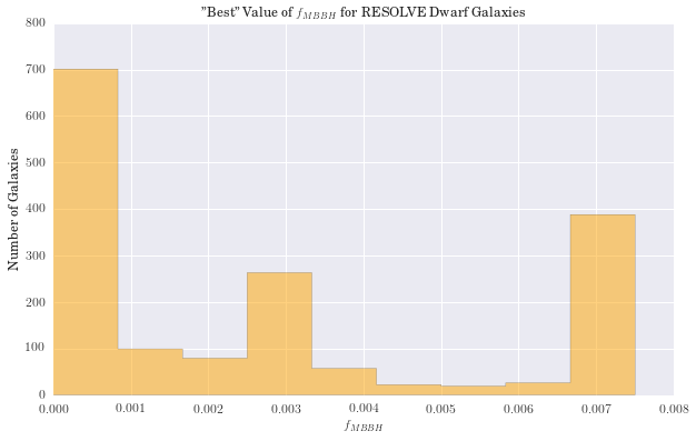
5. Discussion of Results
- We have constructed a Bayesian model that uses an SPS model (BPASS) to explore galaxies with both single and binary star populations.
- We have explored the basic effect of including binary stars and compared these results with data from the RESOLVE survey.
- In addition, we were interested to see if the likelihood of these models favored dwarf galaxies as possible locations for super massive binary black holes, like the progenitors of the LIGO gravitational wave detection event reported earlier this year.
Outcomes:
- We have shown that our model provides similar estimates for galaxy masses when compared to those from the RESOLVE catalog (calculated using Bruzual-Charlot SPS models).
- We have shown that model parameters behave smoothly as a function of binary fraction, \(\alpha\). In general, the model predicts a larger galaxy mass for larger binary fractions.
- Our work with the binary fraction indicates that binary star populations are important for characterizing dwarf galaxies (47% of total stellar population is in binaries). This would indicate that it is favorable for finding LIGO-like progenitors, if only because we expect a significant number of binaries.
- The model also points to metallicities in the neighborhood of 0.013, which is thought to be too large for the formation of LIGO like progenitors (for comparison, \(Z_{\odot} = 0.0134\)).
- Our model, when extended across all galaxies, suggests that the most likely fraction of massive binary black progenitors that could lead to a LIGO-like event is at or below 0.1%. Such a low number is expected; however, our results are preliminary and need to be evaluated more rigorously (i.e., without point estimates).
Future Work:
- Incorporate SPS models with continuous star formation (available from BPASS, but we did not go down the rabbit hole).
- Comparison to other popular SPS models. This was an intended goal from the outset, but it took longer than expected to get comfortable working with the BPASS models.
- Figure out how to use slice sampling/NUTS. This was not a significant component of our final analysis, but it would be interesting to see how well each can do on a large parameter space (even if it remains a discrete grid of parameters).
- Use a more rigorous method to find the distribution of $f_{MBBH}$ (marginalization, combining individual distributions).
6. References
[1] Eldridge, J.J., Izzard, R.G., and C.A. Tout. MNRAS, Volume 384, Issue 3, 1109-1118 (2008).
[2] Eldridge, J.J. and E.R. Stanway. MNRAS, Volume 400, Issue 2, 1019-1028 (2009).
[3] Eldridge, J.J. and E.R. Stanway. MNRAS, Volume 462, Issue 3, 3302-3313 (2016).
[4] B. P. Abbott et al. (LIGO Scientific Collaboration and Virgo Collaboration), Phys. Rev. Lett. 116, 061102 (2016).
[5] RESOLVE: Eckert et al., Astrophysical Journal, 810, 166 (2015).
[6] Belczynski et al., Nature 534, 512–515 (2016)
[7] Hoffman, M.D. and A. Gelman, Journal of Machine Learning Research 15, 1351-1381 (2014).
Initial Mass Function Image by JohannesBuchner - Own work, CC BY-SA 4.0