Titanic: Machine Learning from Disaster
An Exploration into the Data using Python
Data Science on the Hill (Michael Hoffman and Charlies Bonfield)
Table of Contents:
- Introduction
- Loading/Examining the Data
- All the Features!
3a. Extracting Titles from Names
3b. Treating Missing Ports of Departure
3c. Handling Missing Fares
3d. Cabin Number: Relevant or Not?
3e. Quick Fixes
3f. Imputing Missing Ages - Prediction
1. Introduction
To get familiar with Kaggle competitions we worked on the initial tutorial project. The goal is to predict who onboard the Titanic survived the accident. In our initial analysis, we wanted to see how much the predictions would change when the input data was scaled properly as opposed to unscaled (violating the assumptions of the underlying SVM model). We saw an approximately five percent improvement in accuracy by preprocessing the data properly.
# data analysis and wrangling
import pandas as pd
import numpy as np
import scipy

# visualization
import matplotlib.pyplot as plt
import seaborn as sns

# machine learning
from sklearn.svm import SVC
from sklearn import preprocessing
import fancyimpute
from sklearn.model_selection import train_test_split
from sklearn.model_selection import RandomizedSearchCV
from sklearn.metrics import classification_report
from sklearn.model_selection import cross_val_score

%matplotlib inline
2. Loading/Examining the Data
# Load the data.
training_data = pd.read_csv('train.csv')
test_data = pd.read_csv('test.csv')
# Examine the first few rows of data in the training set.
training_data.head()
| PassengerId | Survived | Pclass | Name | Sex | Age | SibSp | Parch | Ticket | Fare | Cabin | Embarked | |
|---|---|---|---|---|---|---|---|---|---|---|---|---|
| 0 | 1 | 0 | 3 | Braund, Mr. Owen Harris | male | 22.0 | 1 | 0 | A/5 21171 | 7.2500 | NaN | S |
| 1 | 2 | 1 | 1 | Cumings, Mrs. John Bradley (Florence Briggs Th... | female | 38.0 | 1 | 0 | PC 17599 | 71.2833 | C85 | C |
| 2 | 3 | 1 | 3 | Heikkinen, Miss. Laina | female | 26.0 | 0 | 0 | STON/O2. 3101282 | 7.9250 | NaN | S |
| 3 | 4 | 1 | 1 | Futrelle, Mrs. Jacques Heath (Lily May Peel) | female | 35.0 | 1 | 0 | 113803 | 53.1000 | C123 | S |
| 4 | 5 | 0 | 3 | Allen, Mr. William Henry | male | 35.0 | 0 | 0 | 373450 | 8.0500 | NaN | S |
3. All the Features!
We will be extracting the features with custom functions. This isn’t necessary for all the features for this project, but we want to leave the possibilty for further development open for the future.
3a. Extracting Titles from Names
While the Name feature itself may not appear to be useful at first glance, we can tease out additional features that may be useful for predicting survival on the Titanic. We will extract a Title from each name, as that carries information about social and marital status (which in turn may relate to survival).
# Extract title from names, then assign to one of five classes.
# Function based on code from: https://www.kaggle.com/startupsci/titanic/titanic-data-science-solutions
def add_title(data):
    data['Title'] = data.Name.str.extract(' ([A-Za-z]+)\.', expand=False)
    data.Title = data.Title.replace(['Lady', 'Countess','Capt', 'Col','Don', 'Dr', 'Major',
                                     'Rev', 'Sir', 'Jonkheer', 'Dona'], 'Rare')
    data.Title = data.Title.replace('Mlle', 'Miss')
    data.Title = data.Title.replace('Ms', 'Miss')
    data.Title = data.Title.replace('Mme', 'Mrs')

    # Map from strings to numerical variables.
    title_mapping = {"Mr": 1, "Miss": 2, "Mrs": 3, "Master": 4, "Rare": 5}

    data.Title = data.Title.map(title_mapping)
    data.Title = data.Title.fillna(0)

    return data
3b. Treating Missing Ports of Embarkation
Next, let’s see if there are any rows that are missing ports of embarkation.
missing_emb_training = training_data[pd.isnull(training_data.Embarked) == True]
missing_emb_test = test_data[pd.isnull(test_data.Embarked) == True]
missing_emb_training.head()
| PassengerId | Survived | Pclass | Name | Sex | Age | SibSp | Parch | Ticket | Fare | Cabin | Embarked | |
|---|---|---|---|---|---|---|---|---|---|---|---|---|
| 61 | 62 | 1 | 1 | Icard, Miss. Amelie | female | 38.0 | 0 | 0 | 113572 | 80.0 | B28 | NaN |
| 829 | 830 | 1 | 1 | Stone, Mrs. George Nelson (Martha Evelyn) | female | 62.0 | 0 | 0 | 113572 | 80.0 | B28 | NaN |
missing_emb_test.head()
| PassengerId | Pclass | Name | Sex | Age | SibSp | Parch | Ticket | Fare | Cabin | Embarked |
|---|
We have two passengers in the training set that are missing ports of embarkation, while we are not missing any in the test set. <br>
The features which may allow us to assign a port of embarkation based on the data that we do have are Pclass, Fare, and Cabin. However, since we are missing so much of the Cabin column (more on that later), let’s focus in on the other two.
grid = sns.FacetGrid(training_data[training_data.Pclass == 1], col='Embarked', size=2.2, aspect=1.6)
grid.map(plt.hist, 'Fare', alpha=.5, bins=20)
grid.map(plt.axvline, x=80.0, color='red', ls='dashed')
grid.add_legend();
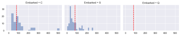
Although Southampton was the most popular port of embarkation, there was a greater fraction of passengers in the first ticket class from Cherbourg who paid 80.00 for their tickets. Therefore, we will assign ‘C’ to the missing values for Embarked. We will also recast Embarked as a numerical feature.
# Recast port of departure as numerical feature.
def simplify_embark(data):
    # Two missing values, assign Cherbourg as port of departure.
    data.Embarked = data.Embarked.fillna('C')

    le = preprocessing.LabelEncoder().fit(data.Embarked)
    data.Embarked = le.transform(data.Embarked)

    return data
3c. Handling Missing Fares
We will perform a similar analysis to see if there are any missing fares.
missing_fare_training = training_data[np.isnan(training_data['Fare'])]
missing_fare_test = test_data[np.isnan(test_data['Fare'])]
missing_fare_training.head()
| PassengerId | Survived | Pclass | Name | Sex | Age | SibSp | Parch | Ticket | Fare | Cabin | Embarked |
|---|
missing_fare_test.head()
| PassengerId | Pclass | Name | Sex | Age | SibSp | Parch | Ticket | Fare | Cabin | Embarked | |
|---|---|---|---|---|---|---|---|---|---|---|---|
| 152 | 1044 | 3 | Storey, Mr. Thomas | male | 60.5 | 0 | 0 | 3701 | NaN | NaN | S |
This time, the Fare column in the training set is complete, but we are missing that information for one passenger in the test set. Since we do have PClass and Embarked, however, we will assign a fare based on the distribution of fares for those particular values of PClass and Embarked.
restricted_training = training_data[(training_data.Pclass == 3) & (training_data.Embarked == 'S')]
restricted_test = test_data[(test_data.Pclass == 3) & (test_data.Embarked == 'S')]
restricted_test = restricted_test[~np.isnan(restricted_test.Fare)] # Leave out poor Mr. Storey
combine = [restricted_training, restricted_test]
combine = pd.concat(combine)

# Find median fare, plot over resulting distribution.
fare_med = np.median(combine.Fare)

sns.kdeplot(combine.Fare, shade=True)
plt.axvline(fare_med, color='r', ls='dashed', lw='1', label='Median')
plt.legend();
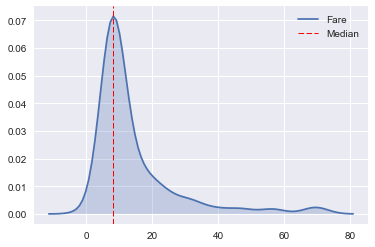
After examining the distribution of Fare restricted to the specified values of Pclass and Fare, we will use the median for the missing fare (as it falls very close the fare corresponding to the peak of the distribution).
test_data['Fare'] = test_data['Fare'].fillna(fare_med)
3d. Cabin Number: Relevant or Not?
When we first encountered the data, we figured that Cabin would be one of the most important features in predicting survival, as it would not be unreasonable to think of it as a proxy for a passenger’s position on the Titanic relative to the lifeboats (distance to deck, distance to nearest stairwell, social class, etc.).
Unfortunately, much of this data is missing:
missing_cabin_training = np.size(training_data.Cabin[pd.isnull(training_data.Cabin) == True]) / np.size(training_data.Cabin) * 100.0
missing_cabin_test = np.size(test_data.Cabin[pd.isnull(test_data.Cabin) == True]) / np.size(test_data.Cabin) * 100.0

print('Percentage of Missing Cabin Numbers (Training): %0.1f' % missing_cabin_training)
print('Percentage of Missing Cabin Numbers (Test): %0.1f' % missing_cabin_test)
Percentage of Missing Cabin Numbers (Training): 77.1
Percentage of Missing Cabin Numbers (Test): 78.2
What can we do with this data (rather, the lack thereof)?
For now, let’s just pull out the first letter of each cabin number (including NaNs), cast them as numbers, and hope they improve the performance of our classifier.
## Set of functions to transform features into more convenient format.
#
# Code performs three separate tasks:
#   (1). Pull out the first letter of the cabin feature.
#          Code taken from: https://www.kaggle.com/jeffd23/titanic/scikit-learn-ml-from-start-to-finish
#   (2). Recasts cabin feature as number.
def simplify_cabins(data):
    data.Cabin = data.Cabin.fillna('N')
    data.Cabin = data.Cabin.apply(lambda x: x[0])

    #cabin_mapping = {'N': 0, 'A': 1, 'B': 1, 'C': 1, 'D': 1, 'E': 1,
    #                 'F': 1, 'G': 1, 'T': 1}
    #data['Cabin_Known'] = data.Cabin.map(cabin_mapping)

    le = preprocessing.LabelEncoder().fit(data.Cabin)
    data.Cabin = le.transform(data.Cabin)

    return data
3e. Quick Fixes
Prior to the last step (which is arguably the largest one), we need to tie up a few remaining loose ends:
- Recast Sex as numerical feature.
- Drop unwanted features.
- Name: We’ve taken out the information that we need (Title).
- Ticket: There appears to be no rhyme or reason to the data in this column, so we remove it from our analysis.
- Combine training/test data prior to age imputation.
# Recast sex as numerical feature.
def simplify_sex(data):
    sex_mapping = {'male': 0, 'female': 1}
    data.Sex = data.Sex.map(sex_mapping).astype(int)

    return data

# Drop all unwanted features (name, ticket).
def drop_features(data):
    return data.drop(['Name','Ticket'], axis=1)

# Perform all feature transformations.
def transform_all(data):
    data = add_title(data)
    data = simplify_embark(data)
    data = simplify_cabins(data)
    data = simplify_sex(data)
    data = drop_features(data)

    return data

training_data = transform_all(training_data)
test_data = transform_all(test_data)

all_data = [training_data, test_data]
combined_data = pd.concat(all_data)
# Inspect data.
combined_data.head()
| Age | Cabin | Embarked | Fare | Parch | PassengerId | Pclass | Sex | SibSp | Survived | Title | |
|---|---|---|---|---|---|---|---|---|---|---|---|
| 0 | 22.0 | 7 | 2 | 7.2500 | 0 | 1 | 3 | 0 | 1 | 0.0 | 1 |
| 1 | 38.0 | 2 | 0 | 71.2833 | 0 | 2 | 1 | 1 | 1 | 1.0 | 3 |
| 2 | 26.0 | 7 | 2 | 7.9250 | 0 | 3 | 3 | 1 | 0 | 1.0 | 2 |
| 3 | 35.0 | 2 | 2 | 53.1000 | 0 | 4 | 1 | 1 | 1 | 1.0 | 3 |
| 4 | 35.0 | 7 | 2 | 8.0500 | 0 | 5 | 3 | 0 | 0 | 0.0 | 1 |
3f. Imputing Missing Ages
It is expected that age will be an important feature; however, a number of ages are missing. Attempting to predict the ages with a simple model was not very successful. We decided to follow the recommendations for imputation from this article.
null_ages = pd.isnull(combined_data.Age)
known_ages = pd.notnull(combined_data.Age)
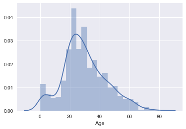
initial_dist = combined_data.Age[known_ages]
# Examine distribution of ages prior to imputation (for comparison).
sns.distplot(initial_dist)
<matplotlib.axes._subplots.AxesSubplot at 0x10acfcb38>
This paper provides an introduction to the MICE method with a focus on practical aspects and challenges in using this method. We have chosen to use the MICE implementation from fancyimpute.
def impute_ages(data):
    drop_survived = data.drop(['Survived'], axis=1)
    column_titles = list(drop_survived)
    mice_results = fancyimpute.MICE().complete(np.array(drop_survived))
    results = pd.DataFrame(mice_results, columns=column_titles)
    results['Survived'] = list(data['Survived'])
    return results

complete_data = impute_ages(combined_data)
complete_data.Age = complete_data.Age[~(complete_data.Age).index.duplicated(keep='first')]
[MICE] Completing matrix with shape (1309, 10)
[MICE] Starting imputation round 1/110, elapsed time 0.001
[MICE] Starting imputation round 2/110, elapsed time 0.005
[MICE] Starting imputation round 3/110, elapsed time 0.006
[MICE] Starting imputation round 4/110, elapsed time 0.007
[MICE] Starting imputation round 5/110, elapsed time 0.008
[MICE] Starting imputation round 6/110, elapsed time 0.009
[MICE] Starting imputation round 7/110, elapsed time 0.010
[MICE] Starting imputation round 8/110, elapsed time 0.010
[MICE] Starting imputation round 9/110, elapsed time 0.011
[MICE] Starting imputation round 10/110, elapsed time 0.012
[MICE] Starting imputation round 11/110, elapsed time 0.013
[MICE] Starting imputation round 12/110, elapsed time 0.014
[MICE] Starting imputation round 13/110, elapsed time 0.015
[MICE] Starting imputation round 14/110, elapsed time 0.016
[MICE] Starting imputation round 15/110, elapsed time 0.017
[MICE] Starting imputation round 16/110, elapsed time 0.018
[MICE] Starting imputation round 17/110, elapsed time 0.019
[MICE] Starting imputation round 18/110, elapsed time 0.020
[MICE] Starting imputation round 19/110, elapsed time 0.021
[MICE] Starting imputation round 20/110, elapsed time 0.022
[MICE] Starting imputation round 21/110, elapsed time 0.023
[MICE] Starting imputation round 22/110, elapsed time 0.023
[MICE] Starting imputation round 23/110, elapsed time 0.024
[MICE] Starting imputation round 24/110, elapsed time 0.025
[MICE] Starting imputation round 25/110, elapsed time 0.026
[MICE] Starting imputation round 26/110, elapsed time 0.027
[MICE] Starting imputation round 27/110, elapsed time 0.028
[MICE] Starting imputation round 28/110, elapsed time 0.028
[MICE] Starting imputation round 29/110, elapsed time 0.029
[MICE] Starting imputation round 30/110, elapsed time 0.030
[MICE] Starting imputation round 31/110, elapsed time 0.034
[MICE] Starting imputation round 32/110, elapsed time 0.035
[MICE] Starting imputation round 33/110, elapsed time 0.036
[MICE] Starting imputation round 34/110, elapsed time 0.037
[MICE] Starting imputation round 35/110, elapsed time 0.038
[MICE] Starting imputation round 36/110, elapsed time 0.039
[MICE] Starting imputation round 37/110, elapsed time 0.040
[MICE] Starting imputation round 38/110, elapsed time 0.040
[MICE] Starting imputation round 39/110, elapsed time 0.041
[MICE] Starting imputation round 40/110, elapsed time 0.042
[MICE] Starting imputation round 41/110, elapsed time 0.043
[MICE] Starting imputation round 42/110, elapsed time 0.044
[MICE] Starting imputation round 43/110, elapsed time 0.044
[MICE] Starting imputation round 44/110, elapsed time 0.045
[MICE] Starting imputation round 45/110, elapsed time 0.046
[MICE] Starting imputation round 46/110, elapsed time 0.047
[MICE] Starting imputation round 47/110, elapsed time 0.048
[MICE] Starting imputation round 48/110, elapsed time 0.050
[MICE] Starting imputation round 49/110, elapsed time 0.050
[MICE] Starting imputation round 50/110, elapsed time 0.051
[MICE] Starting imputation round 51/110, elapsed time 0.052
[MICE] Starting imputation round 52/110, elapsed time 0.053
[MICE] Starting imputation round 53/110, elapsed time 0.054
[MICE] Starting imputation round 54/110, elapsed time 0.055
[MICE] Starting imputation round 55/110, elapsed time 0.056
[MICE] Starting imputation round 56/110, elapsed time 0.056
[MICE] Starting imputation round 57/110, elapsed time 0.057
[MICE] Starting imputation round 58/110, elapsed time 0.058
[MICE] Starting imputation round 59/110, elapsed time 0.059
[MICE] Starting imputation round 60/110, elapsed time 0.060
[MICE] Starting imputation round 61/110, elapsed time 0.061
[MICE] Starting imputation round 62/110, elapsed time 0.062
[MICE] Starting imputation round 63/110, elapsed time 0.063
[MICE] Starting imputation round 64/110, elapsed time 0.064
[MICE] Starting imputation round 65/110, elapsed time 0.065
[MICE] Starting imputation round 66/110, elapsed time 0.066
[MICE] Starting imputation round 67/110, elapsed time 0.067
[MICE] Starting imputation round 68/110, elapsed time 0.068
[MICE] Starting imputation round 69/110, elapsed time 0.069
[MICE] Starting imputation round 70/110, elapsed time 0.070
[MICE] Starting imputation round 71/110, elapsed time 0.070
[MICE] Starting imputation round 72/110, elapsed time 0.071
[MICE] Starting imputation round 73/110, elapsed time 0.072
[MICE] Starting imputation round 74/110, elapsed time 0.073
[MICE] Starting imputation round 75/110, elapsed time 0.074
[MICE] Starting imputation round 76/110, elapsed time 0.075
[MICE] Starting imputation round 77/110, elapsed time 0.076
[MICE] Starting imputation round 78/110, elapsed time 0.077
[MICE] Starting imputation round 79/110, elapsed time 0.077
[MICE] Starting imputation round 80/110, elapsed time 0.078
[MICE] Starting imputation round 81/110, elapsed time 0.079
[MICE] Starting imputation round 82/110, elapsed time 0.080
[MICE] Starting imputation round 83/110, elapsed time 0.081
[MICE] Starting imputation round 84/110, elapsed time 0.082
[MICE] Starting imputation round 85/110, elapsed time 0.083
[MICE] Starting imputation round 86/110, elapsed time 0.083
[MICE] Starting imputation round 87/110, elapsed time 0.084
[MICE] Starting imputation round 88/110, elapsed time 0.085
[MICE] Starting imputation round 89/110, elapsed time 0.086
[MICE] Starting imputation round 90/110, elapsed time 0.087
[MICE] Starting imputation round 91/110, elapsed time 0.088
[MICE] Starting imputation round 92/110, elapsed time 0.088
[MICE] Starting imputation round 93/110, elapsed time 0.089
[MICE] Starting imputation round 94/110, elapsed time 0.090
[MICE] Starting imputation round 95/110, elapsed time 0.091
[MICE] Starting imputation round 96/110, elapsed time 0.092
[MICE] Starting imputation round 97/110, elapsed time 0.093
[MICE] Starting imputation round 98/110, elapsed time 0.093
[MICE] Starting imputation round 99/110, elapsed time 0.094
[MICE] Starting imputation round 100/110, elapsed time 0.095
[MICE] Starting imputation round 101/110, elapsed time 0.096
[MICE] Starting imputation round 102/110, elapsed time 0.097
[MICE] Starting imputation round 103/110, elapsed time 0.098
[MICE] Starting imputation round 104/110, elapsed time 0.099
[MICE] Starting imputation round 105/110, elapsed time 0.100
[MICE] Starting imputation round 106/110, elapsed time 0.101
[MICE] Starting imputation round 107/110, elapsed time 0.102
[MICE] Starting imputation round 108/110, elapsed time 0.102
[MICE] Starting imputation round 109/110, elapsed time 0.103
[MICE] Starting imputation round 110/110, elapsed time 0.104
# Examine distribution of ages after imputation (for comparison).
sns.distplot(initial_dist, label='Initial Distribution')
sns.distplot(complete_data.Age, label='After Imputation')
plt.title('Distribution of Ages')
plt.legend()
<matplotlib.legend.Legend at 0x10c63f710>
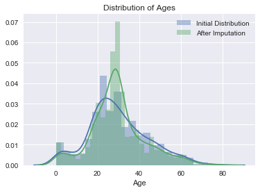
From the output above it is easy to see that distribution is not dramatically altered by the imputation. Additionally, there are no non-sensical ages (negative or extremely old) produced in the process. For experimenting with the tutorial this step is sufficent. In a more serious project this may be one of the most critical steps.
4. Prediction
The model was chosen to be a support vector machine (SVM) model. The reason for this choice:
- the method is for supervised classification.
- effective for high dimensional systems (we intend to expand the features in the next post)
In this model we choose to use the rbf kernel which is essentially an expansion to an “infinite” hyperspace of Gaussians. Therefore, if there is a why to seperate the data points by a single boundary this method has a chance to find it.
Below is the code that impliments the model. The commented code below was used to perform a parameter search to find an optimal fit to the data. The highest ranked outcome was used. There is no particular reason for using a random search -we were just experimenting with the tools availiable natively in sci-kit learn. In fact, it is likely faster to use a straigt-forward grid search for a problem with so few features; however, this random search will be more practical as the number of hyper parameters in future models grows.
# Transform age and fare data to have mean zero and variance 1.0.
scaler = preprocessing.StandardScaler()
select = 'Age Fare'.split()
complete_data[select] = scaler.fit_transform(complete_data[select])

training_data = complete_data[:891]
test_data = complete_data[891:].drop('Survived', axis=1)

# ----------------------------------
# Support Vector Machines
droplist = 'Survived PassengerId'.split()
data = training_data.drop(droplist, axis=1)
# Define features and target values
X, y = data, training_data['Survived']
X_train, X_test, y_train, y_test = train_test_split(X, y, test_size=0.5, random_state=0)

#
# # Set the parameters by cross-validation
# param_dist = {'C': scipy.stats.uniform(0.1, 1000), 'gamma': scipy.stats.uniform(.001, 1.0),
#   'kernel': ['rbf'], 'class_weight':['balanced', None]}
#
# clf = SVC()
#
# # run randomized search
# n_iter_search = 10000
# random_search = RandomizedSearchCV(clf, param_distributions=param_dist,
#                                    n_iter=n_iter_search, n_jobs=-1, cv=4)
#
# start = time()
# random_search.fit(X, y)
# print("RandomizedSearchCV took %.2f seconds for %d candidates"
#       " parameter settings." % ((time() - start), n_iter_search))
# report(random_search.cv_results_)
# exit()

"""
RandomizedSearchCV took 4851.48 seconds for 10000 candidates parameter settings.
Model with rank: 1
Mean validation score: 0.833 (std: 0.013)
Parameters: {'kernel': 'rbf', 'C': 107.54222939713921, 'gamma': 0.013379109762586716, 'class_weight': None}

Model with rank: 2
Mean validation score: 0.832 (std: 0.012)
Parameters: {'kernel': 'rbf', 'C': 154.85033872208422, 'gamma': 0.010852578446979289, 'class_weight': None}

Model with rank: 2
Mean validation score: 0.832 (std: 0.012)
Parameters: {'kernel': 'rbf', 'C': 142.60506747360913, 'gamma': 0.011625955252680842, 'class_weight': None}
"""

params = {'kernel': 'rbf', 'C': 107.54222939713921, 'gamma': 0.013379109762586716, 'class_weight': None}
clf = SVC(**params)
scores = cross_val_score(clf, X, y, cv=4, n_jobs=-1)
print("Accuracy: %0.2f (+/- %0.2f)" % (scores.mean(), scores.std() * 2))

droplist = 'PassengerId'.split()
clf.fit(X,y)
predictions = clf.predict(test_data.drop(droplist, axis=1))
#print(predictions)
print('Predicted Number of Survivors: %d' % int(np.sum(predictions)))
Accuracy: 0.83 (+/- 0.02)
Predicted Number of Survivors: 162
# output .csv for upload
# submission = pd.DataFrame({
#         "PassengerId": test_data['PassengerId'].astype(int),
#         "Survived": predictions.astype(int)
#     })
#
# submission.to_csv('../submission.csv', index=False)
Summary of Results
The base model is gubbed the gender model. It predicts that all women survive and all men don’t. The second model is the SVM model above without scaling on the fare and age features. Finally, the last model is the fully scaled SVM. The results are summarized below, the accuracy is that on the test set withheld by Kaggle:
- gender only: 76.5%
- SVM non-scaled: 75.6%
- SVM scaled: 79.9%
The modest increase over the the base model is enough to move from the lowest rank (gender only model) to the top 15%.
It will clearly be necessary to generate additional informative features to make further progress. We didn’t focus much on the children in the problem (except through age). It may prove fruitful to leverage the sibling and parent information into a new index feature.